Computer Graphics

Output Primitives (Hearn and Baker – Chapter 3)

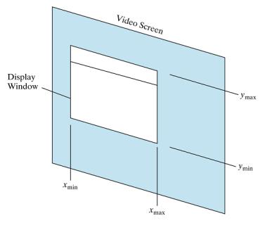
Coordinate Systems

• Object Space
• Image Space
• Normalized

• Absolute
• Relative

Object Space to Image Space Transformations

1. Set up coordinate system and frame of reference in object space (the space in which the real data is found)
2. Get the x,y coordinates of each point
3. Normalize each coordinate to between 0 and 1 by dividing the coordinate by the width or height of the reference frame
4. Scale the normalized value by the width or height of the drawing area.

e.g.

OpenGL

Sample Program

import java.awt.*;

import java.awt.event.*;

import net.java.games.jogl.*;

import net.java.games.jogl.util.*;

public class HBProg2

{

public static void main(String[] args)

{

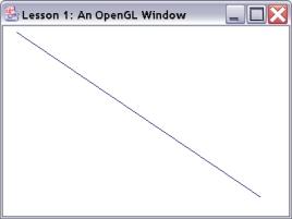
Frame frame = new Frame("Lesson 1: An OpenGL Window");

GLCanvas canvas = GLDrawableFactory.getFactory().createGLCanvas(new GLCapabilities());

canvas.addGLEventListener(new Renderer());

frame.add(canvas);

frame.setSize(400, 300);

frame.addWindowListener(new WindowAdapter()

{

public void windowClosing(WindowEvent e)

{

System.exit(0);

}

});

frame.show();

canvas.requestFocus();

}

static class Renderer implements GLEventListener, KeyListener

{

public void lineSegment (GL gl)

{

gl.glClear (GL.GL_COLOR_BUFFER_BIT); // Set display window to color.

gl.glColor3f (0.0f, 0.0f, 0.75f); // Set line segment color to blue.

gl.glBegin (GL.GL_LINES);

gl.glVertex2i (10, 145);

gl.glVertex2i (180, 15); // Specify line-segment geometry.

gl.glEnd ( );

}

public void display(GLDrawable gLDrawable)

{

final GL gl = gLDrawable.getGL();

gl.glMatrixMode (GL.GL_MODELVIEW);

gl.glLoadIdentity();

lineSegment(gLDrawable.getGL());

}

public void displayChanged(GLDrawable gLDrawable, boolean modeChanged, boolean deviceChanged)

{

}

public void init(GLDrawable gLDrawable)

{

final GL gl = gLDrawable.getGL();

final GLU glu = gLDrawable.getGLU();

gl.glMatrixMode (GL.GL_PROJECTION);

gl.glClearColor (1.0f, 1.0f, 1.0f, 0.0f); //set background to white

glu.gluOrtho2D (0.0, 200.0, 0.0, 150.0); // define drawing area

gLDrawable.addKeyListener(this);

}

public void reshape(GLDrawable gLDrawable, int x, int y, int width, int height)

{

}

public void keyPressed(KeyEvent e)

{

if (e.getKeyCode() == KeyEvent.VK_ESCAPE)

System.exit(0);

}

public void keyReleased(KeyEvent e) {}

public void keyTyped(KeyEvent e) {}

}

}

Points and Lines

Point Plotting

· convert single coordinate position into device positions

· load frame buffer with color code

· low level procedure calls

o setPixel(x,y)

o getPixel(x,y)

OpenGl Points

GlVertex* ( )

glBegin (GL_POINTS);

glVertex* ( );

glEnd ( );

glBegin (GL_POINTS);

glVertex2i (50, 100);

glVertex2i (75, 150);

glVertex2i (100, 200);

glEnd ( );

Can use Arrays to hold points

int point1 [ ] = {50, 100};

int point2 [ ] = {75, 150};

int point3 [ ] = {100, 200};

glBegin (GL_POINTS);

glVertex2iv (point1);

glVertex2iv (point2);

glVertex2iv (point3);

glEnd ( );

Can define point class to define appoint

public class wcPt2D {

float x, y;

};

Then specify a two-dimensional,world-coordinate point position with the statements

wcPt2D pointPos;

pointPos.x = 120.75f;

pointPos.y = 45.30f;

glBegin (GL_POINTS);

glVertex2f (pointPos.x, pointPos.y);

glEnd ( );

Line Drawing

· Calculate intermediate positions along line path between two specified endpoint positions

· Load line color into frame buffer

· Note : true line not at integer values -> aliasing

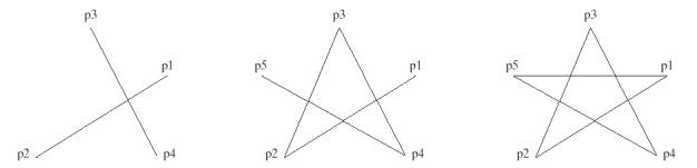
OpenGL Line Drawing

GL_LINES	GL_LINE_STRIP	GL_LINE_LOOP
glBegin (GL_LINES); glVertex2iv (p1); glVertex2iv (p2); glVertex2iv (p3); glVertex2iv (p4); glVertex2iv (p5); glEnd ( );	glBegin (GL_LINE_STRIP); glVertex2iv (p1); glVertex2iv (p2); glVertex2iv (p3); glVertex2iv (p4); glVertex2iv (p5); glEnd ( );	glBegin (GL_LINE_LOOP); glVertex2iv (p1); glVertex2iv (p2); glVertex2iv (p3); glVertex2iv (p4); glVertex2iv (p5); glEnd ( );

Line Drawing Algorithms

· Slope-intercept equation -> y = mx + b

· Use line segments -> (x1,y1) – (x2,y2)

Slope = m = (y2 – y1)/(x2 –x1)

y= [(y2-y1)/(x2-x1)]m +b

· solve for b assuming x1,y1

b = y1 – m x1

· Straight line algorithms based on line equation

o For every interval in x -> Dx, we can compute Dy

o Slope = m = Dy / Dx to give

Dy = m Dx

Dx = Dy / m

· For vector displays Dx, Dy can be set to deflection voltages

o For | m | < 1 set Dx to constant

Dy = m Dx

o For | m | > 1 set Dy to constant

Dx = Dy / m

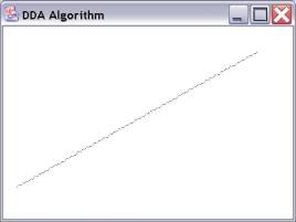
DDA Line drawing Algorithm

· General scan conversion problem: which pixels to turn on

o Assume a line with positive slope in the first octant, i.e., 0.0 <= m <= 1.0.

o Drawn from left to right: (X1, Y1) to (X2, Y2):

o Problem: as xi is incremented to xi+1, which pixel gets turned on - xi+1, yi or xi+1, yi+1?

Digital Differential Analyzer

· Based on calculating Dx or Dy

· Sample line in unit intervals in one direction and calculate increment in other

o Unit steps are always along the coordinate of greatest change

§ e.g. if Dx = 10 and Dy = 5, then take unit steps along x and compute steps along y.

§ Assume a line of positive slope from x1, y1 to x2, y2.

if m <= 1.0 then
 
 let x_step = 1 {dx = 1, dy = 0 or 1}
else {m > 1.0}
 let y_step = 1 {dy = 1, x_step = 0 or 1 }
 

Note: {slope = m = dy/dx}

{m <= 1.0} for x_step = 1, dy = m = yi+1 - yi -> yi+1 = yi + m

{m > 1} for y_step = 1 m = 1/dx => dx = 1/m => xi+1 = xi + 1/m

If, instead, we draw from x2 ,y2 to x1,y1 then:

a.) dx = -1 yi+1 = yi -m or

b.) dy = -1 xi+1 = xi - 1/m

§ For a line with slope < 0.0 and drawing from x1,y1 to x2,y2, i.e., left to right then:

if |m| < 1 then
 let dx = 1 and yi+1 = yi + m
else {|m| ³ 1}
 let dy = -1 and xi+1 = xi -1/m
if draw from x2, y2 to x1, y1 (right to left) then:
 if |m| < 1 then let dx = -1 yi+1 = yi -m
else {|m| ³ 1} dy = 1 xi+1 = xi + 1/m

§ Complete DDA Algorithm

procedure DDA( x1, y1, x2, y2: integer);
var
 dx, dy, steps: integer;
 x_inc, y_inc, x, y: real;
begin
 dx := x2 - x1; dy := y2 - y1;
 if abs(dx) > abs(dy) then
 steps := abs(dx); {steps is larger of dx, dy}
 else
 steps := abs(dy);
 x_inc := dx/steps; y_inc := dy/steps;
 {either x_inc or y_inc = 1.0, the other is the slope}
 x:=x1; y:=y1;
 set_pixel(round(x), round(y));
 for i := 1 to steps do
 begin
 x := x + x_inc;
 y := y + y_inc;
 set_pixel(round(x), round(y));
 end;
end; {DDA}

§ Example

DDA algorithm calculation

xa

ya

xb

yb

dx

dy

step

xinc

yinc

2

0

10

5

8

5

8

1.000

0.625

step

x

y

xs

ys

0

2

0

2

0

1

3.000

0.63

3

1

2

4.000

1.25

4

1

3

5.000

1.88

5

2

4

6.000

2.5

6

3

5

7.000

3.13

7

3

6

8.000

3.75

8

4

7

9.000

4.38

9

4

8

10.000

5

10

5

§ Problems / Concerns:

o Round-off error

o FP calculation time

OpenGL Version of DDA

import java.awt.*;

import java.awt.event.*;

import net.java.games.jogl.*;

import net.java.games.jogl.util.*;

public class DDA

{

public static void main(String[] args)

{

Frame frame = new Frame("Lesson 1: An OpenGL Window");

GLCanvas canvas = GLDrawableFactory.getFactory().createGLCanvas(new GLCapabilities());

canvas.addGLEventListener(new Renderer());

frame.add(canvas);

frame.setSize(400, 300);

frame.addWindowListener(new WindowAdapter()

{

public void windowClosing(WindowEvent e)

{

System.exit(0);

}

});

frame.show();

canvas.requestFocus();

}

static class Renderer implements GLEventListener, KeyListener

{

public void lineDDA (GL gl, int x0, int y0, int xEnd, int yEnd)

{

int dx = xEnd - x0, dy = yEnd - y0, steps, k;

float xIncrement, yIncrement, x = x0, y = y0;

if (Math.abs (dx) > Math.abs (dy))

steps = Math.abs (dx);

else

steps = Math.abs (dy);

xIncrement = (float)dx / (float)steps;

yIncrement = (float)dy / (float) steps;

setpixel (gl, Math.round (x), Math.round (y));

for (k = 0; k < steps; k++) {

x += xIncrement;

y += yIncrement;

setpixel (gl, Math.round (x), Math.round (y));

}

}

public void setpixel(GL gl, int x, int y){

gl.glBegin (GL.GL_POINTS);

gl.glVertex2i (x, y);

gl.glEnd ( );

}

public void display(GLDrawable gLDrawable)

{

final GL gl = gLDrawable.getGL();

gl.glClear (GL.GL_COLOR_BUFFER_BIT); // Set display window to color.

gl.glColor3f (0.0f, 0.0f, 0.75f);

// Set line segment color to blue.

gl.glMatrixMode (GL.GL_MODELVIEW);

gl.glLoadIdentity();

lineDDA(gLDrawable.getGL(), 0,0, 200, 150);

}

public void displayChanged(GLDrawable gLDrawable, boolean modeChanged, boolean deviceChanged)

{

}

public void init(GLDrawable gLDrawable)

{

final GL gl = gLDrawable.getGL();

final GLU glu = gLDrawable.getGLU();

gl.glMatrixMode (GL.GL_PROJECTION);

gl.glClearColor (1.0f, 1.0f, 1.0f, 0.0f); //set background to white

glu.gluOrtho2D (0.0, 200.0, 0.0, 150.0); // define drawing area

gLDrawable.addKeyListener(this);

}

public void reshape(GLDrawable gLDrawable, int x, int y, int width, int height)

{

}

public void keyPressed(KeyEvent e)

{

if (e.getKeyCode() == KeyEvent.VK_ESCAPE)

System.exit(0);

}

public void keyReleased(KeyEvent e) {}

public void keyTyped(KeyEvent e) {}

}

}

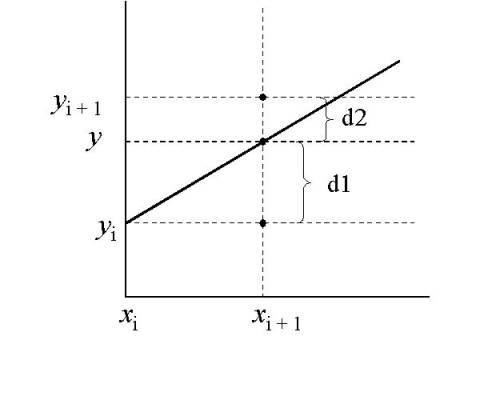
Bresenham (Decision Variable) Method

§ Use incremental integer calculations

§ Makes decision of which is next pixel to turn on

§ Look at the center of the pixels

§ Determine d1 and d2 -> the "error", i.e., the difference from the " true line."

§ d1 and d2 specify an integer parameter whose value is proportional to separation of two pixels

§ Steps in the Bresenham algorithm:

1. Determine the error terms
2. Define a relative error term such that the sign of this term tells which pixel to choose
3. Derive equation to compute successive error terms from first
4. Compute first error term

§ Example | m| < 1

o Sample x at unit intervals

o Start at (x0,y0) and move to (x1, ?)

o Must find y closest to line path

o y is coordinate of true line at xi+1

y = m(xi+1) + b

d1 = y - yi = m(xi+1) + b – yi

d2 = (yi+1) - y = yi+1 -m(xi+1) - b

then d1 - d2 = 2m(xi+1) - 2y + 2b -1

§ now define pi = dx(d1 - d2) = relative error of the two pixels.

§ note: pi < 0 if yi pixel is closer

pi >= 0 if yi+1 pixel is closer

( = 0 is our choice).

§ Therefore we only need to know the sign of pi .

§ With m = dy/dx and substituting in for (d1 - d2) we get

(1) pi = 2 * dy * xi - 2 * dx * yi + 2 * dy + dx * (2 * b - 1)

§ let C = 2 * dy + dx * (2 * b - 1)

· Now look at the relation of p's for successive x terms.

o pi+1 = 2dy * xi+1 - 2 * dx * y i+1 + C

o pi+1 - pi = 2 * dy * (xi+1 - xi) - 2 * dx * ( yi+1 - yi)

with xi+1 = xi + 1 and yi+1= yi + 1 or yi

(2) pi+1 = pi + 2 * dy - 2 * dx(yi+1 -yi)

Note: b = y - dy / dx * x

· Now compute p1 (x1,y1) from (1)

p1 = 2dy * x1 - 2dx * y1 + 2dy + dx(2y1 - 2dy / dx * x1 - 1)

= 2dy * x1 - 2dx * y1 + 2dy + 2dx * y1 - 2dyx1 - dx
= 2dy - dx

· if pi < 0 choose yi and pi+1 = pi + 2dy

· else {pi >= 0} and choose yi+1 so pi+1 = pi + 2dy - 2dx

Bresenham Algorithm for 1st octant:

1. Enter endpoints (x1, y1) and (x2, y2).
2. Display x1, y1.
3. Compute dx = x2 - x1 ; dy = y2 - y1 ; p1 = 2dy - dx.
4. If p1 < 0.0, display (x1 + 1, y1), else display(x1+1, y1 + 1)
5. if p1 < 0.0, p2 = p1 + 2dy else p2 = p1 + 2dy - 2dx
6. Repeat steps 4, 5 until reach (x2, y2).

Note: Only integer Addition and Multiplication by 2. Notice we always increment x by 1.

For a generalized Bresenham Algorithm must look at behavior in different octants.

Worked Example

Bresenham

xa

ya

xb

yb

dx

dy

2dx

2dy

2dy-2dx

20

10

30

18

10

8

20

16

-4

k

pi

xi+1

yi+1

20

10

0

6

21

11

1

2

22

12

2

-2

23

12

3

14

24

13

4

10

25

14

5

6

26

15

6

2

27

16

7

-2

28

16

8

14

29

17

9

10

30

18

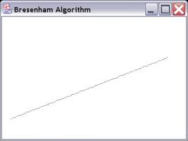
Applet example of DDA and Bresenham

OpenGL version of Bresenham Algorithm

import java.awt.*;

import java.awt.event.*;

import net.java.games.jogl.*;

import net.java.games.jogl.util.*;

public class Bresenham

{

public static void main(String[] args)

{

Frame frame = new Frame("Bresenham Algorithm");

GLCanvas canvas = GLDrawableFactory.getFactory().createGLCanvas(new GLCapabilities());

canvas.addGLEventListener(new Renderer());

frame.add(canvas);

frame.setSize(400, 300);

frame.addWindowListener(new WindowAdapter()

{

public void windowClosing(WindowEvent e)

{

System.exit(0);

}

});

frame.show();

canvas.requestFocus();

}

static class Renderer implements GLEventListener, KeyListener

{

/* Bresenham line-drawing procedure for |m| < 1.0. */

public void lineBres (GL gl, int x0, int y0, int xEnd, int yEnd)

{

int dx = Math.abs(xEnd - x0), dy = Math.abs(yEnd - y0);

int p = 2 * dy - dx;

int twoDy = 2 * dy, twoDyMinusDx = 2 * (dy - dx);

int x, y;

/* Determine which endpoint to use as start position. */

if (x0 > xEnd) {

x = xEnd;

y = yEnd;

xEnd = x0;

}

else {

x = x0;

y = y0;

}

setpixel (gl, x, y);

while (x < xEnd) {

x++;

if (p < 0)

p += twoDy;

else {

y++;

p += twoDyMinusDx;

}

setpixel (gl, x, y);

}

}

public void setpixel(GL gl, int x, int y){

gl.glBegin (GL.GL_POINTS);

gl.glVertex2i (x, y);

gl.glEnd( );

}

public void display(GLDrawable gLDrawable)

{

final GL gl = gLDrawable.getGL();

gl.glClear (GL.GL_COLOR_BUFFER_BIT); // Set display window to color.

gl.glColor3f (0.0f, 0.0f, 0.75f);

// Set line segment color to blue.

gl.glMatrixMode (GL.GL_MODELVIEW);

gl.glLoadIdentity();

lineBres(gLDrawable.getGL(), 10,25, 180, 100);

}

public void displayChanged(GLDrawable gLDrawable, boolean modeChanged, boolean deviceChanged)

{

}

public void init(GLDrawable gLDrawable)

{

final GL gl = gLDrawable.getGL();

final GLU glu = gLDrawable.getGLU();

gl.glMatrixMode (GL.GL_PROJECTION);

gl.glClearColor (1.0f, 1.0f, 1.0f, 0.0f); //set background to white

glu.gluOrtho2D (0.0, 200.0, 0.0, 150.0); // define drawing area

gLDrawable.addKeyListener(this);

}

public void reshape(GLDrawable gLDrawable, int x, int y, int width, int height)

{

}

public void keyPressed(KeyEvent e)

{

if (e.getKeyCode() == KeyEvent.VK_ESCAPE)

System.exit(0);

}

public void keyReleased(KeyEvent e) {}

public void keyTyped(KeyEvent e) {}

}

}

Other Geometric Primitives

Points

P1 (x1, y1, z1)

Line Segments

P1 (x1, y1, z1) -> P2 (x2, y2, z2)

Polyline

Connected line segments

Polygons

Closed polyline where initial and terminal points coincide.

Wireframe models

· Consist of vertices, edges, and polygons (e.g. cube)

· Stored as vertex list, edge listing, polygon listing

Polyhedron

• Closed polygon net
• Encloses a definite volume
• Polygons are faces of volume
• e.g. Platonic solids

Name	n	m	f	v	e
tetrahedron	3	3	4	4	6
hexahedron	4	3	6	8	12
octahedron	3	4	8	6	12
dodecahedron	5	3	12	20	30
icosahedron	3	5	20	12	30
f,v,e: Faces, Vertices, Edges n: edges per face m: faces at each vertex

See Also Visual Geometry Pages

• Problem with polyhedra – takes many polyhedra to approximate smooth surface

Curved Surfaces

• Used for realistic models
• Uses small surface patches instead of polyhedra
• Uses solid modeling from prototype sphere, cone, cylinder, polyhedra => Constructive Solid Geometry (CSG)

Parametric Curves

· A point P(u) on a curve depends on a parameter u.

· Since P(u) also depends on an x coordinate and y coordinate, x and y are functions of u with

P(u) = [ x(u) y(u) ]

· A parametric representation of a straight line is then

P(u) = P₁ + ( P₂ - P₁ ) u where

x(u) = x₁ + ( x₂ - x₁ ) u 0 <= u <= 1

y(u) = y₁ + ( y₂ - y₁ ) u 0 <= u <= 1

· e.g. line from P₁ (2,2) to P₂ (8, 10)

Parametric Equation For Straight Line

from P₁ (2,2) to P₂(8,10)

u	x(u)	y(u)
0.0	2.0	2.0
0.1	2.6	2.8
0.2	3.2	3.6
0.3	3.8	4.4
0.4	4.4	5.2
0.5	5.0	6.0
0.6	5.6	6.8
0.7	6.2	7.6
0.8	6.8	8.4
0.9	7.4	9.2
1.0	8.0	10.0

· e.g. Circle

x(u) = r cos (2 p u)

y(u) = r sin (2 p u)

o Unit circle varying u in increments of 0.05 from 0 to 1.

o Beginning with P₁ (1,0) on the x axis, the circle is built by counterclockwise rotation of point P₁ in 2pu (360 degrees u) increments

Parametric Equation For Circle of Radius 2.0

u	x(u)	y(u)
0.00	2.00	0.00
0.05	1.90	0.62
0.10	1.62	1.18
0.15	1.18	1.62
0.20	0.62	1.90
0.25	0.00	2.00
0.30	-0.62	1.90
0.35	-1.18	1.62
0.40	-1.62	1.18
0.45	-1.90	0.62
0.50	-2.00	0.00
0.55	-1.90	-0.62
0.60	-1.62	-1.18
0.65	-1.18	-1.62
0.70	-0.62	-1.90
0.75	0.00	-2.00
0.80	0.62	-1.90
0.85	1.18	-1.62
0.90	1.62	-1.18
0.95	1.90	-0.62
1.00	2.00	0.00

Curve Design

· Given n + 1 points => find curve which fits shape

• Interpolation
• Approximation

· Try modeling curves using segments +> use linear combination of basis functions

· Usually use polynomials => easy to use

· Polynomials of degree n

_· Continuous piecewise polynomial Q(x) of degree n is a set of k polynomials q(x), each of degree n and k+1 knots (nodes) t₀, …, t_{k ,}such that

Q(x) = q_i(x) for all t_i <= x <= t_i+1 for i = 0, …, k-1

· Polynomials must match or piece together at knots, so…

q_i-1(t_I ) = q_i-1(t_i), i = 0, …, k-1

· Most useful polynomials are cubic (n =3)

Common Basis Functions

· e.g. Bezier Curve

· Bézier curve is a polynomial curve the shape of which is determined by the placement of a series of control points.

· Figure displays a series of Bézier curves with four control points.

· Curves begin with a definition of P(u) as

0 <= u = 1

· B_i are the control points

· J_n,i are the basis or blending functions which assure the curve travels smoothly from B₀ to B₃ .

· Four vertices define a cubic equation with four blending functions.

· This gives

J_3,0 (u) = ( 1 - u )³

J_3,1 (u) = 3 u ( 1 - u )²

J_3,2 (u) = 3 u² ( 1 - u )

J_3,3 (u) = u³

· P(u) becomes

P(u) = B₀ ( 1 - u )³ + B₁ (3 u ( 1 - u )² ) + B₂ (3 u² ( 1 - u )) + B₃ u³

_· x(u) and y(u) are calculated by substituting in the x and y coordinates of B₀ through B₃, respectively_.

· Values for u are selected in a uniform way.

· Figure was calculated with B₀ = (1,1), B₁ = (2,3), B₂ = (4,3), and B₃ = (3,1) and varying u from 0 to 1 in 0.05 increments

Bézier Curve for

B₀(1,1), B₁(2,3), B₂(4,3), B₃(3,1)

u	P(x)	P(y)
0.00	1.00	1.00
0.05	1.16	1.29
0.10	1.33	1.54
0.15	1.50	1.77
0.20	1.69	1.96
0.25	1.88	2.13
0.30	2.06	2.26
0.35	2.25	2.37
0.40	2.42	2.44
0.45	2.59	2.49
0.50	2.75	2.50
0.55	2.89	2.49
0.60	3.02	2.44
0.65	3.12	2.37
0.70	3.20	2.26
0.75	3.25	2.13
0.80	3.27	1.96
0.85	3.26	1.77
0.90	3.21	1.54
0.95	3.13	1.29
1.00	3.00	1.00

Quadric Surfaces

· Sphere

Parametric form:

· Ellipsoid

Parametric form:

See also Visual Geometry pages

· Torus

See also Visual Geometry page

Parametric Form:

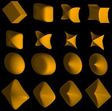
· Superquadrics

o Super ellipse

o s = parameter

o Parametric equations:

o Super ellipsoid

Parametric equation:

Setting a Pixel

· Initial Task: Turning on a pixel (loading the frame buffer/bit-map)

· Assume the simplest case, i.e., an 8-bit, non-interlaced graphics system.

· Then each byte in the frame buffer corresponds to a pixel in the output display.

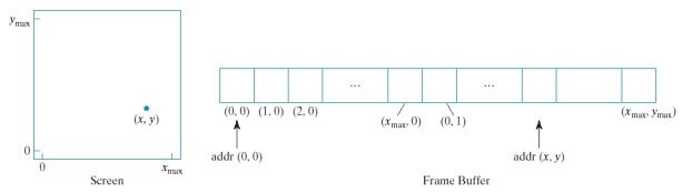
· To find the address of a particular pixel (X,Y):

addr(X, Y) = addr(0,0) + Y rows * (Xm + 1) + X (all in bytes)

o addr(X,Y) = the memory address of pixel (X,Y)

o addr(0,0) = the memory address of the initial pixel (0,0)

o Number of rows = number of raster lines.

o Number of columns = number of pixels/raster line.

· Example:

For a system with 640 × 480 pixel resolution, find the address of pixel X = 340, Y = 150

addr(340, 150) = addr(0,0) + 150 * 640 (bytes/row) + 340

= base + 96,340 is the byte location

Pixel Addressing and Object Geometry

Object Description:

o World description –

o precise coordinate positions

o infinitesimally small mathematical points

o Pixel Coordinates

o Finite screen areas

Aligning Approaches

1. Adjust dimensions of displayed objects to account for amount of overlap of pixel areas with object boundaries

2. Map world coordinates onto screen positions between pixels to align object boundaries with pixel boundaries instead of centers

Screen Grid Coordinates

o Use horizontal/vertical pixel boundary lines instead of centers

Old Way -Pixels are line intersections New Way -Pixels are areas

Maintaining Geometric Properties of Displayed Objects

· Geometric objects are transformed into pixels

· Must account for finite size when transformed to screen

· Say, we have a line from (20,10) to (30,18)

· Line precisely ends in real world at (30,18)

· Pixel extends beyond line

· Must plot pixels from (20,10) to (29,17) to remain on interior

· Same is true for Rectangle

· Vertices at (0,0), (4,0), (4,3), (0,3)

POLYGONS

Polygon

• A plane figure specified by a set of three or more coordinate positions, called vertices, that are connected in sequence by straight-line segments called the edges or sides of the polygon.
• In basic geometry, the polygon edges must have no common point other than their endpoints.
• A polygon must have all its vertices within a single plane and there can be no edge crossings.

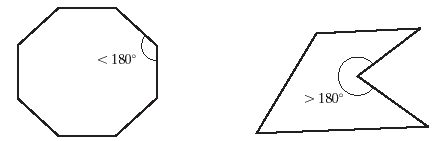
Convex polygon – all interior angles of a polygon are less than or equal to 180 degrees.

Concave polygon –

• at least one interior angles of a polygon is greater than 180 degrees.
• extension of some edges of a concave polygon will intersect other edges
• somepair of interior points will produce a line segment that intersects the polygon boundary

Concave Polygon identification algorithm

• Set up a vector for each polygon edge
• Use the cross product of adjacent edges to test for concavity.
• All vector products will be of the same sign (positive or negative) for a convex polygon.

o If z – value of some cross products is positive while others are negative, concave polygon exits.

(assume no three successive vertices are collinear => gives 0 crossproduct)

Example:

z-component processing

(E1 X E2) > 0

(E2 X E3) > 0

(E3 X E4) < 0

(E4 X E5) > 0

(E5 X E6) > 0

(E6 X E7) > 0

§ Cross product:

V1 X V2 = u |V1||V2| sinq

where u is unit vector perpendicular to V1 and V2

V1 X V2 = ( V1y V2z – V1z V2y, V1z V2x – V1x V2z, V1x V2y – V1y V2x )

Splitting Concave Polygons

E1 = (1, 0, 0)

E2 = (1, 1, 0)

E3 = (1, -1, 0)

E4 = (0, 3, 0)

E5 = (-3, 0, 0)

E6 = (0, -3, 0)

(E1 X E2) = (0, 0, 1)

(E2 X E3) = (0, 0, -2)

(E3 X E4) = (0, 0, 3)

(E4 X E5) = (0, 0, 9)

(E5 X E6) = (0, 0, 9)

(E6 X E1) = (0, 0, 3)

Since E2 X E3 z-value < 0 – must split polygon along line E2

Must determine intersection of line with edge E4

Use slope-intercept form of line:

y = m_ax + b_a y = m_bx + b_b

m_ax + b_a = m_bx + b_b

x = ( b_b - b_a ) / (m_a - m_b )

and

x = ( y - b_a ) / m_a x = ( y – b_b ) / m_b

( y - b_a ) / m_a = ( y – b_b ) / m_b

y = (m_a b_b – m_b b_a ) / (m_a - m_b )

§ Alternative method for splitting concave polygons

1. Rotational Method:

2. Proceed counterclockwise

3. Translate each polygon vertex Vk in sequence to origin

4. Rotate cloackwise so next vertex is on x axis

5. If next vector Vk+2 is below axis, polygon is concave

e.g.

§ can fined, since (x, y=0), substitute into

x = x1 + ( y – y₁ ) / m

so…

x = x1 - y₁ / m

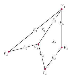
Polygon Tables

VERTEX TABLE

V1 : x1 , y1 , z1

V2 : x2 , y2 , z2

V3 : x3 , y3 , z3

V4 : x4 , y4 , z4

V5 : x5 , y5 , z5

EDGE TABLE

1 : 1 , 2

2 : 2 , 3

3 : 3 , 1

4 : 3 , 4

5 : 4 , 5

6 : 5 , 1

SURFACE-FACET TABLE

S 1 : 1 , 2 , 3

S 2 : 3 , 4 , 5 , 6

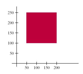
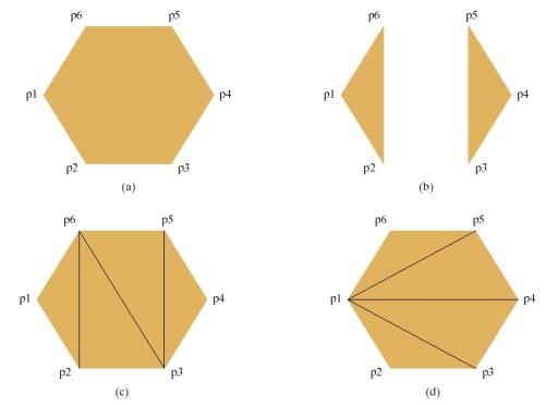
OpenGL Polygon Fill-Area Functions

glRect* (x1,y1,x2,y2);

e.g.

glRecti (200,100,50,250);

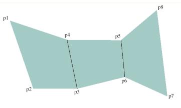
glBegin (GL_POLYGON); glVertex2iv (p1); glVertex2iv (p2); glVertex2iv (p3); glVertex2iv (p4); glVertex2iv (p5); glVertex2iv (p6); glEnd ( );	glBegin (GL_TRIANGLES); glVertex2iv (p1); glVertex2iv (p2); glVertex2iv (p6); glVertex2iv (p3); glVertex2iv (p4); glVertex2iv (p5); glEnd ( );
glBegin (GL_TRIANGLE_STRIP); glVertex2iv (p1); glVertex2iv (p2); glVertex2iv (p6); glVertex2iv (p3); glVertex2iv (p5); glVertex2iv (p4); glEnd ( );	glBegin (GL_TRIANGLE_FAN); glVertex2iv (p1); glVertex2iv (p2); glVertex2iv (p3); glVertex2iv (p4); glVertex2iv (p5); glVertex2iv (p6); glEnd ( );

glBegin (GL_QUADS); glVertex2iv (p1); glVertex2iv (p2); glVertex2iv (p3); glVertex2iv (p4); glVertex2iv (p5); glVertex2iv (p6); glVertex2iv (p7); glVertex2iv (p8); glEnd ( );

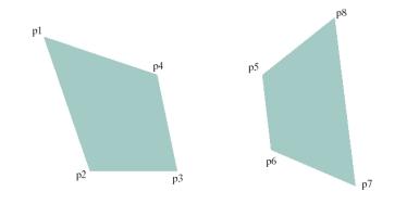
glBegin (GL_QUAD_STRIP); glVertex2iv (p1); glVertex2iv (p2); glVertex2iv (p4); glVertex2iv (p3); glVertex2iv (p5); glVertex2iv (p6); glVertex2iv (p8); glVertex2iv (p7); glEnd ( );