Computer Graphics

Visible-Surface Detection Methods

Classification of Visible-Surface Detection Algorithms

Object-space methods
Image-space methods

Back-Face Detection

· Object space algorithm: Back-Face removal

· No faces on the back of the object are displayed.

· In general - about half of objects faces are back faces

· Algorithm will remove about half of the total polygons in the image.

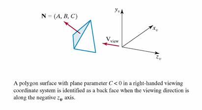
NOTE: Right Handed coordinate System

If n·V > 0 then polygon is backface

n·V = |n| |V| cos q

cos q = n·V / (|n| |V|)

where |n| and |V| are the magnitudes of the vector

|V| = sqrt( V_x² + V_y² + V_z² )

Determining Surface Normal
	x	y	z
1	0.750	0.250	0.000
2	0.250	0.750	0.000
3	0.125	0.750	0.217
4	0.375	0.250	0.650

	center	0.438	0.500	0.108
Point 2 - 1	P	-0.500	0.500	0.000
Point 3 - 2	Q	-0.125	0.000	0.217
Magnitude of P	\|P\|	0.7071
Magnitude of Q	\|Q\|	0.2500
	P(Norm)	-0.7071	0.7071	0.0000
	Q(Norm)	-0.5000	0.0000	0.8660
	Normal Vector	nx	ny	nz
	CrossProd (PxQ)	0.1083	0.1083	0.0625
	n(Norm)	0.6547	0.6547	0.3780

cos RQ	0.00	cos RP	0.00
\|n\|	0.165359	L(n)	1

RlS = (RxSx+RySy+RzSz)=\|R\|\|S\|cosθ

R=PxQ
Rx = PyQz - PzQy
Ry = PzQx -PxQz
Rz = PxQy - PyQx

Standard equation of a plane in 3 space :

Ax + By + Cz + D = 0

Normal to the plane is the vector (A,B,C).

Given three points in space (x1,y1,z1), (x2,y2,z2), (x3,y3,z3) the equation of the plane through these points is given by

Ax1 + By1 + Cz1 + D = 0

Ax2 + By2 + Cz2 + D = 0

Ax3 + By3 + Cz3 + D = 0

in counter-clockwise order, and solving for

A’x_k + B’y_k + C’z_k = 1

where k = 1,2.3

A’ = -(A/D), B’ = -(B/D), and C’ = -(C/D)

Use Cramer’s rule for solving simultaneous equations:

Begin with a system of linear equations, for example, a system involving three variables -

A’x1 + B’y1 + C’z1 = 1

A’x2 + B’y2 + C’z2 = 1

A’x3 + B’y3 + C’z3 = 1

that may be expressed in matrix form as

Here the coordinates constitute a coefficient matrix (A) and the vector components (A’,B’,C’) are the unknowns.

Generally, this is written as

a₁₁x + a₁₂ y = c₁a₂₁x + a₂₂ y = c₂

for the 2D case and expressed in matrix form

the square matrix A, with real number entries,

can be expressed by a real number called the determinant of the matrix.

The determinant is written as -

and is defined by det A = a₁₁a₂₂ - a₁₂a₂₂

There are two other matrices obtained by replacing the coefficients in each column by the constants c₁ and c₂ respectively

Their determinants are det A_x and det A_y respectively.

For a 3 x 3 matrix of coefficients the determinant may be expressed as either:

or as a cofactor expansion

Cramer's Rule states that

For our system, the result is

Expanding the above gives
A = y1 (z2 - z3) + y2 (z3 - z1) + y3 (z1 - z2)
B = z1 (x2 - x3) + z2 (x3 - x1) + z3 (x1 - x2)
C = x1 (y2 - y3) + x2 (y3 - y1) + x3 (y1 - y2)
D = -x1 (y2 z3 - y3 z2) - x2 (y3 z1 - y1 z3) - x3 (y1 z2 - y2 z1)

If the 3 points are collinear then the normal (A,B,C) will be (0,0,0).

The sign of S = Ax + By + Cz + D determines which side the point (x,y,z) lies with respect to the plane.

· If s > 0 then the point lies on the same side as the normal (A,B,C).

· If s < 0 then it lies on the opposite side

· If s = 0 then the point (x,y,z) lies on the plane.

Calculating Normal using plane equations
		X	y	z
Original Data	1	0.750	0.250	0.000
	2	0.250	0.750	0.000
	3	0.125	0.750	0.217
	4	0.375	0.250	0.650

use 3 points in succession
	A	0.1083
	B	0.1083
	C	0.0625
	D	-0.1083
	S	0.171

Same as with normal vector

Back-Face detection Procedure

Limitations:

Used only for solid objects modeled as a polygon mesh.
Problematic for concave polyhedra.

e.g. partially hidden face will not be eliminated by Back-face removal.

Depth-Buffer Method

· Image-Space Algorithm also known as z-buffer method

· Test z - depth of each surface to determine the surface closest to observer.

o Declare an array z buffer(x, y) with one entry for each pixel position.

o Initialize array to the maximum depth.

o The algorithm is:

for each polygon P

  for each pixel (x, y) in P

    compute z_depth at x, y

    if z_depth < z_buffer (x, y) then

       set_pixel (x, y, color)

       z_buffer (x, y) <= z_depth

· Polygon scan-conversion procedure is modified to add the z-buffer test.

- At a surface position (x,y) the depth is calculated from the plane equation:

- the depth of the next position z’ becomes, for each successive position along scanline:

note: A/C is a constant, so successive z values are only an addition

Possible algorithm:

1.Begin at top vertex of polygon

2.Recursively calculate x-coordinate values down left edge of polygon

3.Subsequent x-values for each scanline calculated from starting x-value

and depth values become

· Advantage

Always works and is simple to implement => used in hardware

· Disadvantages

o Large memory requirements

o E.g. (640 x 480 )

§ real (4 bytes): 4bytes/pixel = 1,228,000 bytes.

§ usually use a 24-bit z-buffer = 900,000 bytes

§ may need additional z - buffers for special effects, e.g. shadows.

A-Buffer Method

· Extension of z-buffer -> accumulation buffer

· Each buffer position can reference a linked-list of surfaces

· Allows pixel color to be computed as combination of surface colors for transparency, anti-aliasing, etc.

· Each position has 2 fields:

1.depth field – real number

2.surface data field

If depth field >= 0

depth at pixel location stored

Surface color and pixel coverage

else

(multiple surface contributions to pixel color)

surface color filed contains pointer to linked list of surface data comprising:

· RGB intensity components

· Opacity parameter

· Depth

· Percent of area coverage

· Surface identifier

· Other surface rendering parameters

Depth Sorting Methods

Painter's Algorithm

· Based on depth sorting

· Object space algorithm

Sort all polygons according to z value

Simplest to use maximum z value

Draw polygons from back (maximum z) to front (minimum z)

· Problems with simple Painter's algorithm:

· P’ has a greater depth than P

· P’ will be drawn first.

· P’ and P intersect

BSP-Tree Method

· A binary space partitioning tree (bsp–tree) is a binary tree whose nodes contain polygons.

· Binary space partitioning, or BSP, divides space into distinct sections by building a tree representing that space.

· Used to sort polygons.

· A BSP takes the polygons and divides them into two groups bychoosing a plane, usually taken from the set of polygons, and divides the world into two spaces.

· It decides which side of the plane each polygon is on, or it may also be on the plane.

· If a polygon intersects the splitting plane it must be split into two separate polygons, one on each side of the plane.

· The tree is built by choosing a partitioning plane and dividing the remaining polygons into two or three lists: Front, Back and On lists – done by comparing the normal vector of the plane with that of each polygon.

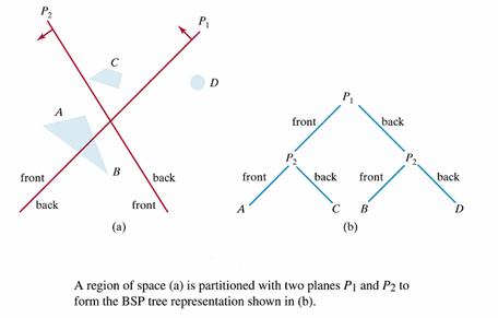
· For each node in a bsp-tree the polygons in the left subtree lie behind the polygon at the node while the polygons in the right subtree lie in front of the polygon at the node.

· Each polygon has a fixed normal vector, and front and back are measured relative to this fixed normal.

· Once a bsp-tree is constructed for a scene, the polygons are rendered by an in order traversal of the bsp-tree.

· Recursive algorithms for generating a bsp-tree and then using the bsp-tree to render a scene are presented below.

Algorithm for Generating a BSP–Tree

Select any polygon (plane) in the scene for the root.
Partition all the other polygons in the scene to the back (left subtree) or the front (right subtree).
Split any polygons lying on both sides of the root (see below).
Build the left and right subtrees recursively.

BSP-Tree Rendering Algorithm (In order tree traversal)

If the eye is in front of the root, then

Display the left subtree (behind)

Display the root

Display the right subtree (front)

If eye is in back of the root, then

Display the right subtree (front)

Display the root

Display the left subtree (back)

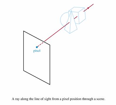
Ray Casting Method

· The ray casting algorithm for hidden surfaces employs no special data structures.

· A ray is fired from the eye through each pixel on the screen in order to locate the polygon in the scene closest to the eye.

· The color and intensity of this polygon is displayed at the pixel.

Ray casting is easy to implement for polygonal models because the only calculation required is the intersection of a line with a plane.

Ray Casting Algorithm

Through each pixel, fire a ray to the eye:
Intersect the ray with each polygonal plane.
Reject intersections that lie outside the polygon.
Accept the closest remaining intersection -- that is, the intersection with the smallest value of the parameter along the line.

The main advantage of the ray casting algorithm for hidden surfaces is that ray casting can be used even with non-polygonal surfaces.
All that is needed to implement the ray casting algorithm for hidden surfaces is a line/surface intersection algorithm for each distinct surface type.
The main disadvantage of ray casting is that the method is slow. Ray casting is a brute force technique that makes no use of pixel coherence.