Chapter 4. Communication
Interprocess communication
is at the heart of all distributed systems. It makes no sense to study
distributed systems without carefully examining the ways that processes on
different machines can exchange information. Communication in distributed
systems is always based on low-level message passing as offered by the
underlying network. Expressing communication through message passing is harder
than using primitives based on shared memory, as available for nondistributed
platforms. Modern distributed systems often consist of thousands or even
millions of processes scattered across a network with unreliable communication
such as the Internet. Unless the primitive communication facilities of computer
networks are replaced by something else, development of large-scale distributed
applications is extremely difficult.
In this chapter, we start by
discussing the rules that communicating processes must adhere to, known as
protocols, and concentrate on structuring those protocols in the form of
layers. We then look at three widely-used models for communication: Remote
Procedure Call (RPC), Message-Oriented Middleware (MOM), and data streaming. We
also discuss the general problem of sending data to multiple receivers, called
multicasting.
Our first model for
communication in distributed systems is the remote procedure call (RPC). An RPC
aims at hiding most of the intricacies of message passing, and is ideal for
client-server applications.
In many distributed applications,
communication does not follow the rather strict pattern of client-server
interaction. In those cases, it turns out that thinking in terms of messages is
more appropriate. However, the low-level communication facilities of computer
networks are in many ways not suitable due to their lack of distribution
transparency. An alternative is to use a high-level message-queuing model, in
which communication proceeds much the same as in electronic mail systems.
Message-oriented middleware (MOM) is a subject important enough to warrant a
section of its own.
[Page 116]
With the advent of
multimedia distributed systems, it became apparent that many systems were
lacking support for communication of continuous media, such as audio and video.
What is needed is the notion of a stream that can support the continuous flow
of messages, subject to various timing constraints. Streams are discussed in a
separate section.
Finally, since our
understanding of setting up multicast facilities has improved, novel and elegant
solutions for data dissemination have emerged. We pay separate attention to
this subject in the last section of this chapter.
4.1. Fundamentals
Before we start our
discussion on communication in distributed systems, we first recapitulate some
of the fundamental issues related to communication. In the next section we
briefly discuss network communication protocols, as these form the basis for
any distributed system. After that, we take a different approach by classifying
the different types of communication that occurs in distributed systems.
4.1.1. Layered Protocols
Due to the absence of shared
memory, all communication in distributed systems is based on sending and
receiving (low level) messages. When process A wants to communicate with
process B, it first builds a message in its own address space. Then it executes
a system call that causes the operating system to send the message over the
network to B. Although this basic idea sounds simple enough, in order to
prevent chaos, A and B have to agree on the meaning of the bits being sent. If
A sends a brilliant new novel written in French and encoded in IBM's EBCDIC
character code, and B expects the inventory of a supermarket written in English
and encoded in ASCII, communication will be less than optimal.
Many different agreements
are needed. How many volts should be used to signal a 0-bit, and how many volts
for a 1-bit? How does the receiver know which is the last bit of the message?
How can it detect if a message has been damaged or lost, and what should it do
if it finds out? How long are numbers, strings, and other data items, and how
are they represented? In short, agreements are needed at a variety of levels,
varying from the low-level details of bit transmission to the high-level
details of how information is to be expressed.
[Page 117]
To make it easier to deal
with the numerous levels and issues involved in communication, the
International Standards Organization (ISO) developed a reference model that
clearly identifies the various levels involved, gives them standard names, and
points out which level should do which job. This model is called the Open
Systems Interconnection Reference Model (Day and Zimmerman, 1983), usually
abbreviated as ISO OSI or sometimes just the OSI model. It should be emphasized
that the protocols that were developed as part of the OSI model were never
widely used and are essentially dead now. However, the underlying model itself
has proved to be quite useful for understanding computer networks. Although we
do not intend to give a full description of this model and all of its
implications here, a short introduction will be helpful. For more details, see
Tanen-baum (2003).
The OSI model is designed to
allow open systems to communicate. An open system is one that is prepared to
communicate with any other open system by using standard rules that govern the
format, contents, and meaning of the messages sent and received. These rules
are formalized in what are called protocols. To allow a group of computers to
communicate over a network, they must all agree on the protocols to be used. A
distinction is made between two general types of protocols. With connection
oriented protocols, before exchanging data the sender and receiver first
explicitly establish a connection, and possibly negotiate the protocol they
will use. When they are done, they must release (terminate) the connection. The
telephone is a connection-oriented communication system. With connectionless
protocols, no setup in advance is needed. The sender just transmits the first
message when it is ready. Dropping a letter in a mailbox is an example of
connectionless communication. With computers, both connection-oriented and
connectionless communication are common.
In the OSI model,
communication is divided up into seven levels or layers, as shown in Fig. 4-1.
Each layer deals with one specific aspect of the communication. In this way,
the problem can be divided up into manageable pieces, each of which can be
solved independent of the others. Each layer provides an interface to the one
above it. The interface consists of a set of operations that together define
the service the layer is prepared to offer its users.
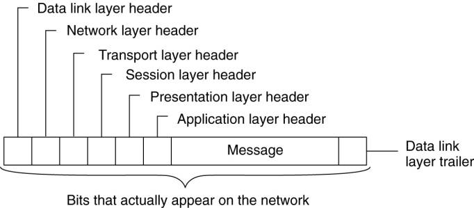
Figure 4-1. Layers,
interfaces, and protocols in the OSI model.
(This item is displayed on
page 118 in the print version)

When process A on machine 1
wants to communicate with process B on machine 2, it builds a message and
passes the message to the application layer on its machine. This layer might be
a library procedure, for example, but it could also be implemented in some
other way (e.g., inside the operating system, on an external network processor,
etc.). The application layer software then adds a header to the front of the
message and passes the resulting message across the layer 6/7 interface to the
presentation layer. The presentation layer in turn adds its own header and
passes the result down to the session layer, and so on. Some layers add not
only a header to the front, but also a trailer to the end. When it hits the
bottom, the physical layer actually transmits the message (which by now might
look as shown in Fig. 4-2) by putting it onto the physical transmission medium.
[Page 118]
Figure 4-2. A typical
message as it appears on the network.
When the message arrives at
machine 2, it is passed upward, with each layer stripping off and examining its
own header. Finally, the message arrives at the receiver, process B, which may
reply to it using the reverse path. The information in the layer n header is
used for the layer n protocol.
As an example of why layered
protocols are important, consider communication between two companies, Zippy
Airlines and its caterer, Mushy Meals, Inc. Every month, the head of passenger
service at Zippy asks her secretary to contact the sales manager's secretary at
Mushy to order 100,000 boxes of rubber chicken. Traditionally, the orders went
via the post office. However, as the postal service deteriorated, at some point
the two secretaries decided to abandon it and communicate by e-mail. They could
do this without bothering their bosses, since their protocol deals with the
physical transmission of the orders, not their contents.
[Page 119]
Similarly, the head of
passenger service can decide to drop the rubber chicken and go for Mushy's new
special, prime rib of goat, without that decision affecting the secretaries.
The thing to notice is that we have two layers here, the bosses and the
secretaries. Each layer has its own protocol (subjects of discussion and technology)
that can be changed independently of the other one. It is precisely this
independence that makes layered protocols attractive. Each one can be changed
as technology improves, without the other ones being affected.
In the OSI model, there are
not two layers, but seven, as we saw in Fig. 4-1. The collection of protocols
used in a particular system is called a protocol suite or protocol stack. It is
important to distinguish a reference model from its actual protocols. As we
mentioned, the OSI protocols were never popular. In contrast, protocols
developed for the Internet, such as TCP and IP, are mostly used. In the
following sections, we will briefly examine each of the OSI layers in turn,
starting at the bottom. However, instead of giving examples of OSI protocols,
where appropriate, we will point out some of the Internet protocols used in
each layer.
Lower-Level Protocols
We start with discussing the
three lowest layers of the OSI protocol suite. Together, these layers implement
the basic functions that encompass a computer network.
The physical layer is
concerned with transmitting the 0s and 1s. How many volts to use for 0 and 1,
how many bits per second can be sent, and whether transmission can take place
in both directions simultaneously are key issues in the physical layer. In
addition, the size and shape of the network connector (plug), as well as the
number of pins and meaning of each are of concern here.
The physical layer protocol
deals with standardizing the electrical, mechanical, and signaling interfaces
so that when one machine sends a 0 bit it is actually received as a 0 bit and
not a 1 bit. Many physical layer standards have been developed (for different
media), for example, the RS-232-C standard for serial communication lines.
The physical layer just
sends bits. As long as no errors occur, all is well. However, real
communication networks are subject to errors, so some mechanism is needed to
detect and correct them. This mechanism is the main task of the data link
layer. What it does is to group the bits into units, sometimes called frames,
and see that each frame is correctly received.
The data link layer does its
work by putting a special bit pattern on the start and end of each frame to
mark them, as well as computing a checksum by adding up all the bytes in the
frame in a certain way. The data link layer appends the checksum to the frame.
When the frame arrives, the receiver recomputes the checksum from the data and
compares the result to the checksum following the frame. If the two agree, the
frame is considered correct and is accepted. It they disagree, the receiver
asks the sender to retransmit it. Frames are assigned sequence numbers (in the
header), so everyone can tell which is which.
[Page 120]
On a LAN, there is usually no
need for the sender to locate the receiver. It just puts the message out on the
network and the receiver takes it off. A wide-area network, however, consists
of a large number of machines, each with some number of lines to other
machines, rather like a large-scale map showing major cities and roads
connecting them. For a message to get from the sender to the receiver it may
have to make a number of hops, at each one choosing an outgoing line to use.
The question of how to choose the best path is called routing, and is
essentially the primary task of the network layer.
The problem is complicated
by the fact that the shortest route is not always the best route. What really
matters is the amount of delay on a given route, which, in turn, is related to
the amount of traffic and the number of messages queued up for transmission
over the various lines. The delay can thus change over the course of time. Some
routing algorithms try to adapt to changing loads, whereas others are content
to make decisions based on long-term averages.
At present, the most widely
used network protocol is the connectionless IP (Internet Protocol), which is
part of the Internet protocol suite. An IP packet (the technical term for a
message in the network layer) can be sent without any setup. Each IP packet is
routed to its destination independent of all others. No internal path is
selected and remembered.
Transport Protocols
The transport layer forms
the last part of what could be called a basic network protocol stack, in the
sense that it implements all those services that are not provided at the
interface of the network layer, but which are reasonably needed to build
network applications. In other words, the transport layer turns the underlying
network into something that an application developer can use.
Packets can be lost on the
way from the sender to the receiver. Although some applications can handle
their own error recovery, others prefer a reliable connection. The job of the
transport layer is to provide this service. The idea is that the application
layer should be able to deliver a message to the transport layer with the
expectation that it will be delivered without loss.
Upon receiving a message
from the application layer, the transport layer breaks it into pieces small
enough for transmission, assigns each one a sequence number, and then sends
them all. The discussion in the transport layer header concerns which packets
have been sent, which have been received, how many more the receiver has room
to accept, which should be retransmitted, and similar topics.
Reliable transport
connections (which by definition are connection oriented) can be built on top
of connection-oriented or connectionless network services. In the former case
all the packets will arrive in the correct sequence (if they arrive at all),
but in the latter case it is possible for one packet to take a different route
and arrive earlier than the packet sent before it. It is up to the transport
layer software to put everything back in order to maintain the illusion that a
transport connection is like a big tube—you put messages into it and they come
out undamaged and in the same order in which they went in. Providing this
end-to-end communication behavior is an important aspect of the transport
layer.
[Page 121]
The Internet transport
protocol is called TCP (Transmission Control Protocol) and is described in
detail in Comer (2006). The combination TCP/IP is now used as a de facto
standard for network communication. The Internet protocol suite also supports a
connectionless transport protocol called UDP (Universal Datagram Protocol),
which is essentially just IP with some minor additions. User programs that do
not need a connection-oriented protocol normally use UDP.
Additional transport
protocols are regularly proposed. For example, to support real-time data
transfer, the Real-time Transport Protocol (RTP) has been defined. RTP is a
framework protocol in the sense that it specifies packet formats for real-time
data without providing the actual mechanisms for guaranteeing data delivery. In
addition, it specifies a protocol for monitoring and controlling data transfer
of RTP packets (Schulzrinne et al., 2003).
Higher-Level Protocols
Above the transport layer,
OSI distinguished three additional layers. In practice, only the application
layer is ever used. In fact, in the Internet protocol suite, everything above
the transport layer is grouped together. In the face of middle-ware systems, we
shall see in this section that neither the OSI nor the Internet approach is really
appropriate.
The session layer is
essentially an enhanced version of the transport layer. It provides dialog
control, to keep track of which party is currently talking, and it provides
synchronization facilities. The latter are useful to allow users to insert
checkpoints into long transfers, so that in the event of a crash, it is
necessary to go back only to the last checkpoint, rather than all the way back
to the beginning. In practice, few applications are interested in the session
layer and it is rarely supported. It is not even present in the Internet
protocol suite. However, in the context of developing middleware solutions, the
concept of a session and its related protocols has turned out to be quite
relevant, notably when defining higher-level communication protocols.
Unlike the lower layers,
which are concerned with getting the bits from the sender to the receiver
reliably and efficiently, the presentation layer is concerned with the meaning
of the bits. Most messages do not consist of random bit strings, but more
structured information such as people's names, addresses, amounts of money, and
so on. In the presentation layer it is possible to define records containing
fields like these and then have the sender notify the receiver that a message contains
a particular record in a certain format. This makes it easier for machines with
different internal representations to communicate with each other.
[Page 122]
The OSI application layer was
originally intended to contain a collection of standard network applications
such as those for electronic mail, file transfer, and terminal emulation. By
now, it has become the container for all applications and protocols that in one
way or the other do not fit into one of the underlying layers. From the
perspective of the OSI reference model, virtually all distributed systems are
just applications.
What is missing in this
model is a clear distinction between applications, application-specific
protocols, and general-purpose protocols. For example, the Internet File
Transfer Protocol (FTP) (Postel and Reynolds, 1985; and Horowitz and Lunt,
1997) defines a protocol for transferring files between a client and server
machine. The protocol should not be confused with the ftp program, which is an
end-user application for transferring files and which also (not entirely by
coincidence) happens to implement the Internet FTP.
Another example of a typical
application-specific protocol is the HyperText Transfer Protocol (HTTP)
(Fielding et al., 1999), which is designed to remotely manage and handle the
transfer of Web pages. The protocol is implemented by applications such as Web
browsers and Web servers. However, HTTP is now also used by systems that are
not intrinsically tied to the Web. For example, Java's object-invocation
mechanism uses HTTP to request the invocation of remote objects that are
protected by a firewall (Sun Microsystems, 2004b).
There are also many
general-purpose protocols that are useful to many applications, but which
cannot be qualified as transport protocols. In many cases, such protocols fall
into the category of middleware protocols, which we discuss next.
Middleware Protocols
Middleware is an application
that logically lives (mostly) in the application layer, but which contains many
general-purpose protocols that warrant their own layers, independent of other,
more specific applications. A distinction can be made between high-level
communication protocols and protocols for establishing various middleware
services.
There are numerous protocols
to support a variety of middleware services. For example, as we discuss in
Chap. 9, there are various ways to establish authentication, that is, provide
proof of a claimed identity. Authentication protocols are not closely tied to
any specific application, but instead, can be integrated into a middleware
system as a general service. Likewise, authorization protocols by which
authenticated users and processes are granted access only to those resources for
which they have authorization, tend to have a general, application-independent
nature.
As another example, we shall
consider a number of distributed commit protocols in Chap. 8. Commit protocols
establish that in a group of processes either all processes carry out a
particular operation, or that the operation is not carried out at all. This
phenomenon is also referred to as atomicity and is widely applied in
transactions. As we shall see, besides transactions, other applications, like
fault-tolerant ones, can also take advantage of distributed commit protocols.
[Page 123]
As a last example, consider
a distributed locking protocol by which a resource can be protected against
simultaneous access by a collection of processes that are distributed across
multiple machines. We shall come across a number of such protocols in Chap. 6.
Again, this is an example of a protocol that can be used to implement a general
middleware service, but which, at the same time, is highly independent of any
specific application.
Middleware communication
protocols support high-level communication services. For example, in the next
two sections we shall discuss protocols that allow a process to call a
procedure or invoke an object on a remote machine in a highly transparent way.
Likewise, there are high-level communication services for setting and
synchronizing streams for transferring real-time data, such as needed for
multimedia applications. As a last example, some middleware systems offer
reliable multicast services that scale to thousands of receivers spread across
a wide-area network.
Some of the middleware
communication protocols could equally well belong in the transport layer, but
there may be specific reasons to keep them at a higher level. For example,
reliable multicasting services that guarantee scalability can be implemented
only if application requirements are taken into account. Consequently, a
middleware system may offer different (tunable) protocols, each in turn
implemented using different transport protocols, but offering a single
interface.
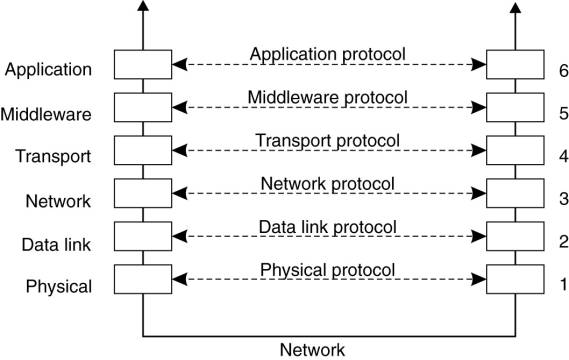
Taking this approach to
layering leads to a slightly adapted reference model for communication, as
shown in Fig. 4-3. Compared to the OSI model, the session and presentation
layer have been replaced by a single middleware layer that contains
application-independent protocols. These protocols do not belong in the lower
layers we just discussed. The original transport services may also be offered
as a middleware service, without being modified. This approach is somewhat
analogous to offering UDP at the transport level. Likewise, middleware
communication services may include message-passing services comparable to those
offered by the transport layer.
[Page 124]
Figure 4-3. An adapted
reference model for networked communication.
(This item is displayed on
page 123 in the print version)
In the remainder of this
chapter, we concentrate on four high-level middle-ware communication services:
remote procedure calls, message queuing services, support for communication of continuous
media through streams, and multicasting. Before doing so, there are other
general criteria for distinguishing (middleware) communication which we discuss
next.
4.1.2. Types of
Communication
To understand the various
alternatives in communication that middleware can offer to applications, we
view the middleware as an additional service in client-server computing, as
shown in Fig. 4-4. Consider, for example an electronic mail system. In
principle, the core of the mail delivery system can be seen as a middleware
communication service. Each host runs a user agent allowing users to compose,
send, and receive e-mail. A sending user agent passes such mail to the mail
delivery system, expecting it, in turn, to eventually deliver the mail to the
intended recipient. Likewise, the user agent at the receiver's side connects to
the mail delivery system to see whether any mail has come in. If so, the
messages are transferred to the user agent so that they can be displayed and
read by the user.
Figure 4-4. Viewing
middleware as an intermediate (distributed) service in application-level
communication.
An electronic mail system is
a typical example in which communication is persistent. With persistent
communication, a message that has been submitted for transmission is stored by
the communication middleware as long as it takes to deliver it to the receiver.
In this case, the middleware will store the message at one or several of the
storage facilities shown in Fig. 4-4. As a consequence, it is not necessary for
the sending application to continue execution after submitting the message.
Likewise, the receiving application need not be executing when the message is
submitted.
[Page 125]
In contrast, with transient
communication, a message is stored by the communication system only as long as
the sending and receiving application are executing. More precisely, in terms
of Fig. 4-4, the middleware cannot deliver a message due to a transmission
interrupt, or because the recipient is currently not active, it will simply be
discarded. Typically, all transport-level communication services offer only
transient communication. In this case, the communication system consists
traditional store-and-forward routers. If a router cannot deliver a message to
the next one or the destination host, it will simply drop the message.
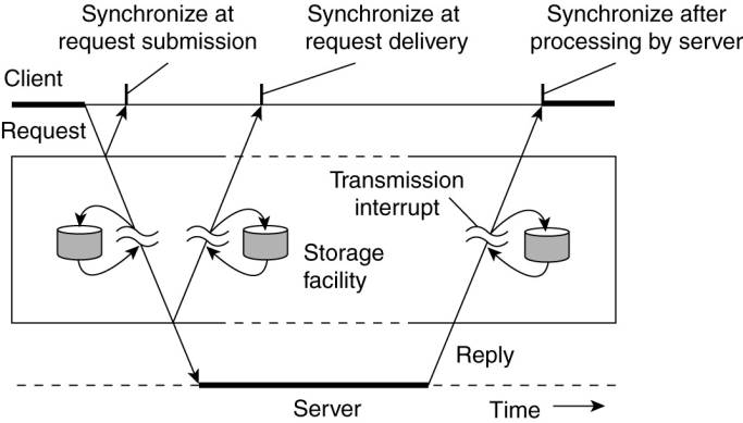
Besides being persistent or
transient, communication can also be asynchronous or synchronous. The
characteristic feature of asynchronous communication is that a sender continues
immediately after it has submitted its message for transmission. This means
that the message is (temporarily) stored immediately by the middleware upon
submission. With synchronous communication, the sender is blocked until its
request is known to be accepted. There are essentially three points where
synchronization can take place. First, the sender may be blocked until the
middleware notifies that it will take over transmission of the request. Second,
the sender may synchronize until its request has been delivered to the intended
recipient. Third, synchronization may take place by letting the sender wait
until its request has been fully processed, that is, up the time that the
recipient returns a response.
Various combinations of
persistence and synchronization occur in practice. Popular ones are persistence
in combination with synchronization at request submission, which is a common
scheme for many message-queuing systems, which we discuss later in this
chapter. Likewise, transient communication with synchronization after the request
has been fully processed is also widely used. This scheme corresponds with
remote procedure calls, which we also discuss below.
Besides persistence and
synchronization, we should also make a distinction between discrete and
streaming communication. The examples so far all fall in the category of
discrete communication: the parties communicate by messages, each message
forming a complete unit of information. In contrast, streaming involves sending
multiple messages, one after the other, where the messages are related to each
other by the order they are sent, or because there is a temporal relationship.
We return to streaming communication extensively below.
4.2. Remote Procedure
Call
Many distributed systems have
been based on explicit message exchange between processes. However, the
procedures send and receive do not conceal communication at all, which is
important to achieve access transparency in distributed systems. This problem
has long been known, but little was done about it until a paper by Birrell and
Nelson (1984) introduced a completely different way of handling communication.
Although the idea is refreshingly simple (once someone has thought of it), the
implications are often subtle. In this section we will examine the concept, its
implementation, its strengths, and its weaknesses.
[Page 126]
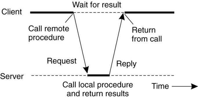
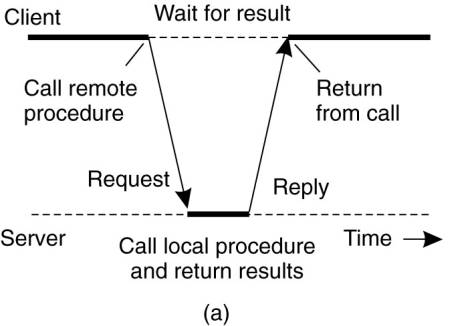
In a nutshell, what Birrell
and Nelson suggested was allowing programs to call procedures located on other
machines. When a process on machine A calls a procedure on machine B, the
calling process on A is suspended, and execution of the called procedure takes
place on B. Information can be transported from the caller to the callee in the
parameters and can come back in the procedure result. No message passing at all
is visible to the programmer. This method is known as Remote Procedure Call, or
often just RPC.
While the basic idea sounds
simple and elegant, subtle problems exist. To start with, because the calling
and called procedures run on different machines, they execute in different
address spaces, which causes complications. Parameters and results also have to
be passed, which can be complicated, especially if the machines are not
identical. Finally, either or both machines can crash and each of the possible
failures causes different problems. Still, most of these can be dealt with, and
RPC is a widely-used technique that underlies many distributed systems.
4.2.1. Basic RPC
Operation
We first start with
discussing conventional procedure calls, and then explain how the call itself
can be split into a client and server part that are each executed on different
machines.
Conventional Procedure Call
To understand how RPC works,
it is important first to fully understand how a conventional (i.e., single
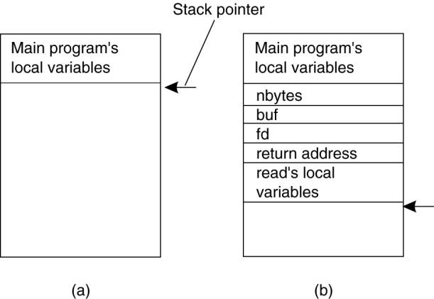
machine) procedure call works. Consider a call in C like
count = read(fd, buf,
nbytes);
where fd is an integer
indicating a file, buf is an array of characters into which data are read, and
nbytes is another integer telling how many bytes to read. If the call is made
from the main program, the stack will be as shown in Fig. 4-5(a) before the
call. To make the call, the caller pushes the parameters onto the stack in
order, last one first, as shown in Fig. 4-5(b). (The reason that C compilers
push the parameters in reverse order has to do with printf—by doing so, printf
can always locate its first parameter, the format string.) After the read
procedure has finished running, it puts the return value in a register, removes
the return address, and transfers control back to the caller. The caller then
removes the parameters from the stack, returning the stack to the original
state it had before the call.
[Page 127]
Figure 4-5. (a) Parameter
passing in a local procedure call: the stack before the call to read. (b) The
stack while the called procedure is active.
Several things are worth
noting. For one, in C, parameters can be call-by-value or call-by-reference. A
value parameter, such as fd or nbytes, is simply copied to the stack as shown
in Fig. 4-5(b). To the called procedure, a value parameter is just an
initialized local variable. The called procedure may modify it, but such
changes do not affect the original value at the calling side.
A reference parameter in C is
a pointer to a variable (i.e., the address of the variable), rather than the
value of the variable. In the call to read, the second parameter is a reference
parameter because arrays are always passed by reference in C. What is actually
pushed onto the stack is the address of the character array. If the called
procedure uses this parameter to store something into the character array, it
does modify the array in the calling procedure. The difference between
call-by-value and call-by-reference is quite important for RPC, as we shall
see.
One other parameter passing
mechanism also exists, although it is not used in C. It is called
call-by-copy/restore. It consists of having the variable copied to the stack by
the caller, as in call-by-value, and then copied back after the call,
overwriting the caller's original value. Under most conditions, this achieves
exactly the same effect as call-by-reference, but in some situations, such as
the same parameter being present multiple times in the parameter list, the semantics
are different. The call-by-copy/restore mechanism is not used in many
languages.
The decision of which
parameter passing mechanism to use is normally made by the language designers
and is a fixed property of the language. Sometimes it depends on the data type
being passed. In C, for example, integers and other scalar types are always
passed by value, whereas arrays are always passed by reference, as we have
seen. Some Ada compilers use copy/restore for in out parameters, but others use
call-by-reference. The language definition permits either choice, which makes
the semantics a bit fuzzy.
[Page 128]
Client and Server Stubs
The idea behind RPC is to
make a remote procedure call look as much as possible like a local one. In
other words, we want RPC to be transparent—the calling procedure should not be
aware that the called procedure is executing on a different machine or vice
versa. Suppose that a program needs to read some data from a file. The
programmer puts a call to read in the code to get the data. In a traditional
(single-processor) system, the read routine is extracted from the library by
the linker and inserted into the object program. It is a short procedure, which
is generally implemented by calling an equivalent read system call. In other words,
the read procedure is a kind of interface between the user code and the local
operating system.
Even though read does a
system call, it is called in the usual way, by pushing the parameters onto the
stack, as shown in Fig. 4-5(b). Thus the programmer does not know that read is
actually doing something fishy.
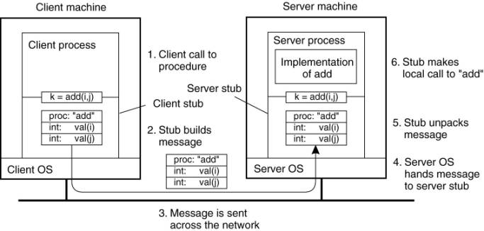
RPC achieves its
transparency in an analogous way. When read is actually a remote procedure
(e.g., one that will run on the file server's machine), a different version of
read, called a client stub, is put into the library. Like the original one, it,
too, is called using the calling sequence of Fig. 4-5(b). Also like the
original one, it too, does a call to the local operating system. Only unlike
the original one, it does not ask the operating system to give it data.
Instead, it packs the parameters into a message and requests that message to be
sent to the server as illustrated in Fig. 4-6. Following the call to send, the
client stub calls receive, blocking itself until the reply comes back.
Figure 4-6. Principle of RPC
between a client and server program.
When the message arrives at
the server, the server's operating system passes it up to a server stub. A
server stub is the server-side equivalent of a client stub: it is a piece of
code that transforms requests coming in over the network into local procedure
calls. Typically the server stub will have called receive and be blocked
waiting for incoming messages. The server stub unpacks the parameters from the
message and then calls the server procedure in the usual way (i.e., as in Fig.
4-5). From the server's point of view, it is as though it is being called
directly by the client—the parameters and return address are all on the stack
where they belong and nothing seems unusual. The server performs its work and
then returns the result to the caller in the usual way. For example, in the
case of read, the server will fill the buffer, pointed to by the second
parameter, with the data. This buffer will be internal to the server stub.
[Page 129]
When the server stub gets
control back after the call has completed, it packs the result (the buffer) in
a message and calls send to return it to the client. After that, the server
stub usually does a call to receive again, to wait for the next incoming request.
When the message gets back
to the client machine, the client's operating system sees that it is addressed
to the client process (or actually the client stub, but the operating system
cannot see the difference). The message is copied to the waiting buffer and the
client process unblocked. The client stub inspects the message, unpacks the
result, copies it to its caller, and returns in the usual way. When the caller
gets control following the call to read, all it knows is that its data are
available. It has no idea that the work was done remotely instead of by the
local operating system.
This blissful ignorance on
the part of the client is the beauty of the whole scheme. As far as it is
concerned, remote services are accessed by making ordinary (i.e., local)
procedure calls, not by calling send and receive. All the details of the
message passing are hidden away in the two library procedures, just as the
details of actually making system calls are hidden away in traditional
libraries.
To summarize, a remote
procedure call occurs in the following steps:
1. The client procedure calls the client
stub in the normal way.
2. The client stub builds a message and
calls the local operating system.
3. The client's OS sends the message to the
remote OS.
4. The remote OS gives the message to the
server stub.
5. The server stub unpacks the parameters
and calls the server.
6. The server does the work and returns the
result to the stub.
7. The server stub packs it in a message
and calls its local OS.
8. The server's OS sends the message to the
client's OS.
9. The client's OS gives the message to the
client stub.
10.
The stub unpacks the result and
returns to the client.
The net effect of all these
steps is to convert the local call by the client procedure to the client stub,
to a local call to the server procedure without either client or server being
aware of the intermediate steps or the existence of the network.
[Page 130]
4.2.2. Parameter Passing
The function of the client
stub is to take its parameters, pack them into a message, and send them to the
server stub. While this sounds straightforward, it is not quite as simple as it
at first appears. In this section we will look at some of the issues concerned
with parameter passing in RPC systems.
Passing Value Parameters
Packing parameters into a
message is called parameter marshaling. As a very simple example, consider a
remote procedure, add(i, j), that takes two integer parameters i and j and returns
their arithmetic sum as a result. (As a practical matter, one would not
normally make such a simple procedure remote due to the overhead, but as an
example it will do.) The call to add, is shown in the left-hand portion (in the
client process) in Fig. 4-7. The client stub takes its two parameters and puts
them in a message as indicated. It also puts the name or number of the
procedure to be called in the message because the server might support several
different calls, and it has to be told which one is required.
Figure 4-7. The steps
involved in a doing a remote computation through RPC.
When the message arrives at
the server, the stub examines the message to see which procedure is needed and
then makes the appropriate call. If the server also supports other remote
procedures, the server stub might have a switch statement in it to select the
procedure to be called, depending on the first field of the message. The actual
call from the stub to the server looks like the original client call, except
that the parameters are variables initialized from the incoming message.
When the server has
finished, the server stub gains control again. It takes the result sent back by
the server and packs it into a message. This message is sent back back to the client
stub, which unpacks it to extract the result and returns the value to the
waiting client procedure.
[Page 131]
As long as the client and
server machines are identical and all the parameters and results are scalar
types, such as integers, characters, and Booleans, this model works fine.
However, in a large distributed system, it is common that multiple machine
types are present. Each machine often has its own representation for numbers,
characters, and other data items. For example, IBM mainframes use the EBCDIC
character code, whereas IBM personal computers use ASCII. As a consequence, it
is not possible to pass a character parameter from an IBM PC client to an IBM
mainframe server using the simple scheme of Fig. 4-7: the server will interpret
the character incorrectly.
Similar problems can occur
with the representation of integers (one's complement versus two's complement)
and floating-point numbers. In addition, an even more annoying problem exists
because some machines, such as the Intel Pentium, number their bytes from right
to left, whereas others, such as the Sun SPARC, number them the other way. The
Intel format is called little endian and the SPARC format is called big endian,
after the politicians in Gulliver's Travels who went to war over which end of
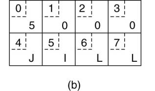
an egg to break (Cohen, 1981). As an example, consider a procedure with two
parameters, an integer and a four-character string. Each parameter requires one
32-bit word. Fig. 4-8(a) shows what the parameter portion of a message built by
a client stub on an Intel Pentium might look like. The first word contains the
integer parameter, 5 in this case, and the second contains the string
"JILL."
Figure 4-8. (a) The original
message on the Pentium. (b) The message after receipt on the SPARC. (c) The message
after being inverted. The little numbers in boxes indicate the address of each
byte.


Since messages are
transferred byte for byte (actually, bit for bit) over the network, the first
byte sent is the first byte to arrive. In Fig. 4-8(b) we show what the message
of Fig. 4-8(a) would look like if received by a SPARC, which numbers its bytes
with byte 0 at the left (high-order byte) instead of at the right (low-order
byte) as do all the Intel chips. When the server stub reads the parameters at addresses
0 and 4, respectively, it will find an integer equal to 83,886,080 (5 x 224)
and a string "JILL".
One obvious, but
unfortunately incorrect, approach is to simply invert the bytes of each word
after they are received, leading to Fig. 4-8(c). Now the integer is 5 and the
string is "LLIJ". The problem here is that integers are reversed by
the different byte ordering, but strings are not. Without additional
information about what is a string and what is an integer, there is no way to
repair the damage.
[Page 132]
Passing Reference Parameters
We now come to a difficult
problem: How are pointers, or in general, references passed? The answer is:
only with the greatest of difficulty, if at all. Remember that a pointer is meaningful
only within the address space of the process in which it is being used. Getting
back to our read example discussed earlier, if the second parameter (the
address of the buffer) happens to be 1000 on the client, one cannot just pass
the number 1000 to the server and expect it to work. Address 1000 on the server
might be in the middle of the program text.
One solution is just to
forbid pointers and reference parameters in general. However, these are so
important that this solution is highly undesirable. In fact, it is not
necessary either. In the read example, the client stub knows that the second
parameter points to an array of characters. Suppose, for the moment, that it
also knows how big the array is. One strategy then becomes apparent: copy the
array into the message and send it to the server. The server stub can then call
the server with a pointer to this array, even though this pointer has a
different numerical value than the second parameter of read has. Changes the
server makes using the pointer (e.g., storing data into it) directly affect the
message buffer inside the server stub. When the server finishes, the original
message can be sent back to the client stub, which then copies it back to the
client. In effect, call-by-reference has been replaced by copy/restore.
Although this is not always identical, it frequently is good enough.
One optimization makes this
mechanism twice as efficient. If the stubs know whether the buffer is an input
parameter or an output parameter to the server, one of the copies can be
eliminated. If the array is input to the server (e.g., in a call to write) it
need not be copied back. If it is output, it need not be sent over in the first
place.
As a final comment, it is
worth noting that although we can now handle pointers to simple arrays and
structures, we still cannot handle the most general case of a pointer to an
arbitrary data structure such as a complex graph. Some systems attempt to deal
with this case by actually passing the pointer to the server stub and generating
special code in the server procedure for using pointers. For example, a request
may be sent back to the client to provide the referenced data.
Parameter Specification and Stub Generation
From what we have explained
so far, it is clear that hiding a remote procedure call requires that the
caller and the callee agree on the format of the messages they exchange, and
that they follow the same steps when it comes to, for example, passing complex
data structures. In other words, both sides in an RPC should follow the same
protocol or the RPC will not work correctly.
[Page 133]
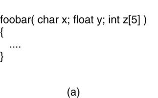
As a simple example,
consider the procedure of Fig. 4-9(a). It has three parameters, a character, a
floating-point number, and an array of five integers. Assuming a word is four
bytes, the RPC protocol might prescribe that we should transmit a character in
the rightmost byte of a word (leaving the next 3 bytes empty), a float as a
whole word, and an array as a group of words equal to the array length,
preceded by a word giving the length, as shown in Fig. 4-9(b). Thus given these
rules, the client stub for foobar knows that it must use the format of Fig.
4-9(b), and the server stub knows that incoming messages for foobar will have
the format of Fig. 4-9(b).
Figure 4-9. (a) A procedure.
(b) The corresponding message.

Defining the message format
is one aspect of an RPC protocol, but it is not sufficient. What we also need
is the client and the server to agree on the representation of simple data structures,
such as integers, characters, Booleans, etc. For example, the protocol could
prescribe that integers are represented in two's complement, characters in
16-bit Unicode, and floats in the IEEE standard #754 format, with everything
stored in little endian. With this additional information, messages can be
unambiguously interpreted.
With the encoding rules now
pinned down to the last bit, the only thing that remains to be done is that the
caller and callee agree on the actual exchange of messages. For example, it may
be decided to use a connection-oriented transport service such as TCP/IP. An
alternative is to use an unreliable datagram service and let the client and
server implement an error control scheme as part of the RPC protocol. In
practice, several variants exist.
Once the RPC protocol has
been fully defined, the client and server stubs need to be implemented.
Fortunately, stubs for the same protocol but different procedures normally
differ only in their interface to the applications. An interface consists of a
collection of procedures that can be called by a client, and which are
implemented by a server. An interface is usually available in the same
programing language as the one in which the client or server is written
(although this is strictly speaking, not necessary). To simplify matters,
interfaces are often specified by means of an Interface Definition Language
(IDL). An interface specified in such an IDL is then subsequently compiled into
a client stub and a server stub, along with the appropriate compile-time or
run-time interfaces.
[Page 134]
Practice shows that using an
interface definition language considerably simplifies client-server
applications based on RPCs. Because it is easy to fully generate client and server
stubs, all RPC-based middleware systems offer an IDL to support application
development. In some cases, using the IDL is even mandatory, as we shall see in
later chapters.
4.2.3. Asynchronous RPC
As in conventional procedure
calls, when a client calls a remote procedure, the client will block until a
reply is returned. This strict request-reply behavior is unnecessary when there
is no result to return, and only leads to blocking the client while it could
have proceeded and have done useful work just after requesting the remote
procedure to be called. Examples of where there is often no need to wait for a
reply include: transferring money from one account to another, adding entries
into a database, starting remote services, batch processing, and so on.
To support such situations,
RPC systems may provide facilities for what are called asynchronous RPCs, by
which a client immediately continues after issuing the RPC request. With
asynchronous RPCs, the server immediately sends a reply back to the client the
moment the RPC request is received, after which it calls the requested
procedure. The reply acts as an acknowledgment to the client that the server is
going to process the RPC. The client will continue without further blocking as
soon as it has received the server's acknowledgment. Fig. 4-10(b) shows how
client and server interact in the case of asynchronous RPCs. For comparison,
Fig. 4-10(a) shows the normal request-reply behavior.
Figure 4-10. (a) The
interaction between client and server in a traditional RPC. (b) The interaction
using asynchronous RPC.
(This item is displayed on
page 135 in the print version)

Asynchronous RPCs can also
be useful when a reply will be returned but the client is not prepared to wait
for it and do nothing in the meantime. For example, a client may want to
prefetch the network addresses of a set of hosts that it expects to contact
soon. While a naming service is collecting those addresses, the client may want
to do other things. In such cases, it makes sense to organize the communication
between the client and server through two asynchronous RPCs, as shown in Fig.
4-11. The client first calls the server to hand over a list of host names that
should be looked up, and continues when the server has acknowledged the receipt
of that list. The second call is done by the server, who calls the client to
hand over the addresses it found. Combining two asynchronous RPCs is sometimes
also referred to as a deferred synchronous RPC.
Figure 4-11. A client and
server interacting through two asynchronous RPCs.
(This item is displayed on
page 135 in the print version)

It should be noted that
variants of asynchronous RPCs exist in which the client continues executing
immediately after sending the request to the server. In other words, the client
does not wait for an acknowledgment of the server's acceptance of the request.
We refer to such RPCs as one-way RPCs. The problem with this approach is that
when reliability is not guaranteed, the client cannot know for sure whether or not
its request will be processed. We return to these matters in Chap. 8. Likewise,
in the case of deferred synchronous RPC, the client may poll the server to see
whether the results are available yet instead of letting the server calling
back the client.
[Page 135]
4.2.4. Example: DCE RPC
Remote procedure calls have
been widely adopted as the basis of middleware and distributed systems in
general. In this section, we take a closer look at one specific RPC system: the
Distributed Computing Environment (DCE), which was developed by the Open
Software Foundation (OSF), now called The Open Group. DCE RPC is not as popular
as some other RPC systems, notably Sun RPC. However, DCE RPC is nevertheless
representative of other RPC systems, and its specifications have been adopted
in Microsoft's base system for distributed computing, DCOM (Eddon and Eddon,
1998). We start with a brief introduction to DCE, after which we consider the
principal workings of DCE RPC. Detailed technical information on how to develop
RPC-based applications can be found in Stevens (1999).
[Page 136]
Introduction to DCE
DCE is a true middleware
system in that it is designed to execute as a layer of abstraction between
existing (network) operating systems and distributed applications. Initially
designed for UNIX, it has now been ported to all major operating systems
including VMS and Windows variants, as well as desktop operating systems. The
idea is that the customer can take a collection of existing machines, add the
DCE software, and then be able to run distributed applications, all without
disturbing existing (nondistributed) applications. Although most of the DCE
package runs in user space, in some configurations a piece (part of the
distributed file system) must be added to the kernel. The Open Group itself
only sells source code, which vendors integrate into their systems.
The programming model
underlying all of DCE is the client-server model, which was extensively
discussed in the previous chapter. User processes act as clients to access remote
services provided by server processes. Some of these services are part of DCE
itself, but others belong to the applications and are written by the
applications programmers. All communication between clients and servers takes
place by means of RPCs.
There are a number of
services that form part of DCE itself. The distributed file service is a
worldwide file system that provides a transparent way of accessing any file in
the system in the same way. It can either be built on top of the hosts' native
file systems or used instead of them. The directory service is used to keep
track of the location of all resources in the system. These resources include
machines, printers, servers, data, and much more, and they may be distributed
geographically over the entire world. The directory service allows a process to
ask for a resource and not have to be concerned about where it is, unless the
process cares. The security service allows resources of all kinds to be
protected, so access can be restricted to authorized persons. Finally, the
distributed time service is a service that attempts to keep clocks on the
different machines globally synchronized. As we shall see in later chapters,
having some notion of global time makes it much easier to ensure consistency in
a distributed system.
Goals of DCE RPC
The goals of the DCE RPC
system are relatively traditional. First and foremost, the RPC system makes it
possible for a client to access a remote service by simply calling a local
procedure. This interface makes it possible for client (i.e., application)
programs to be written in a simple way, familiar to most programmers. It also
makes it easy to have large volumes of existing code run in a distributed
environment with few, if any, changes.
[Page 137]
It is up to the RPC system
to hide all the details from the clients, and, to some extent, from the servers
as well. To start with, the RPC system can automatically locate the correct
server, and subsequently set up the communication between client and server
software (generally called binding). It can also handle the message transport
in both directions, fragmenting and reassembling them as needed (e.g., if one
of the parameters is a large array). Finally, the RPC system can automatically
handle data type conversions between the client and the server, even if they
run on different architectures and have a different byte ordering.
As a consequence of the RPC
system's ability to hide the details, clients and servers are highly
independent of one another. A client can be written in Java and a server in C,
or vice versa. A client and server can run on different hardware platforms and
use different operating systems. A variety of network protocols and data
representations are also supported, all without any intervention from the client
or server.
Writing a Client and a Server
The DCE RPC system consists
of a number of components, including languages, libraries, daemons, and utility
programs, among others. Together these make it possible to write clients and
servers. In this section we will describe the pieces and how they fit together.
The entire process of writing and using an RPC client and server is summarized
in Fig. 4-12.
In a client-server system,
the glue that holds everything together is the interface definition, as specified
in the Interface Definition Language, or IDL. It permits procedure declarations
in a form closely resembling function prototypes in ANSI C. IDL files can also
contain type definitions, constant declarations, and other information needed
to correctly marshal parameters and unmarshal results. Ideally, the interface
definition should also contain a formal definition of what the procedures do,
but such a definition is beyond the current state of the art, so the interface
definition just defines the syntax of the calls, not their semantics. At best
the writer can add a few comments describing what the procedures do.
A crucial element in every
IDL file is a globally unique identifier for the specified interface. The
client sends this identifier in the first RPC message and the server verifies
that it is correct. In this way, if a client inadvertently tries to bind to the
wrong server, or even to an older version of the right server, the server will
detect the error and the binding will not take place.
Interface definitions and
unique identifiers are closely related in DCE. As illustrated in Fig. 4-12, the
first step in writing a client/server application is usually calling the
uuidgen program, asking it to generate a prototype IDL file containing an
interface identifier guaranteed never to be used again in any interface
generated anywhere by uuidgen. Uniqueness is ensured by encoding in it the
location and time of creation. It consists of a 128-bit binary number
represented in the IDL file as an ASCII string in hexadecimal.
[Page 138]
Figure 4-12. The steps in
writing a client and a server in DCE RPC.
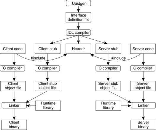
The next step is editing the
IDL file, filling in the names of the remote procedures and their parameters. It
is worth noting that RPC is not totally transparent—for example, the client and
server cannot share global variables—but the IDL rules make it impossible to
express constructs that are not supported.
When the IDL file is
complete, the IDL compiler is called to process it. The output of the IDL
compiler consists of three files:
1. A header file (e.g., interface.h, in C terms).
2. The client stub.
3. The server stub.
The header file contains the
unique identifier, type definitions, constant definitions, and function
prototypes. It should be included (using #include) in both the client and
server code. The client stub contains the actual procedures that the client
program will call. These procedures are the ones responsible for collecting and
packing the parameters into the outgoing message and then calling the runtime
system to send it. The client stub also handles unpacking the reply and
returning values to the client. The server stub contains the procedures called
by the runtime system on the server machine when an incoming message arrives.
These, in turn, call the actual server procedures that do the work.
[Page 139]
The next step is for the
application writer to write the client and server code. Both of these are then
compiled, as are the two stub procedures. The resulting client code and client
stub object files are then linked with the runtime library to produce the
executable binary for the client. Similarly, the server code and server stub
are compiled and linked to produce the server's binary. At runtime, the client
and server are started so that the application is actually executed as well.
Binding a Client to a Server
To allow a client to call a
server, it is necessary that the server be registered and prepared to accept
incoming calls. Registration of a server makes it possible for a client to
locate the server and bind to it. Server location is done in two steps:
1. Locate the server's machine.
2. Locate the server (i.e., the correct
process) on that machine.
The second step is somewhat
subtle. Basically, what it comes down to is that to communicate with a server,
the client needs to know an end point, on the server's machine to which it can
send messages. An end point (also commonly known as a port) is used by the
server's operating system to distinguish incoming messages for different
processes. In DCE, a table of (server, end point) pairs is maintained on each
server machine by a process called the DCE daemon. Before it becomes available
for incoming requests, the server must ask the operating system for an end
point. It then registers this end point with the DCE daemon. The DCE daemon
records this information (including which protocols the server speaks) in the
end point table for future use.
The server also registers
with the directory service by providing it the network address of the server's
machine and a name under which the server can be looked up. Binding a client to
a server then proceeds as shown in Fig. 4-13.
Figure 4-13.
Client-to-server binding in DCE.
(This item is displayed on page
140 in the print version)
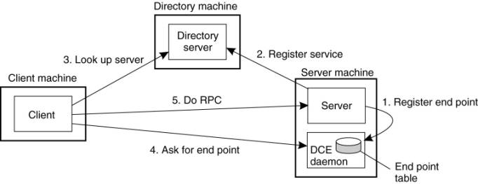
Let us assume that the
client wants to bind to a video server that is locally known under the name
/local/multimedia/video/movies. It passes this name to the directory server,
which returns the network address of the machine running the video server. The
client then goes to the DCE daemon on that machine (which has a well-known end
point), and asks it to look up the end point of the video server in its end
point table. Armed with this information, the RPC can now take place. On
subsequent RPCs this lookup is not needed. DCE also gives clients the ability
to do more sophisticated searches for a suitable server when that is needed.
Secure RPC is also an option where confidentiality or data integrity is
crucial.
[Page 140]
Performing an RPC
The actual RPC is carried
out transparently and in the usual way. The client stub marshals the parameters
to the runtime library for transmission using the protocol chosen at binding
time. When a message arrives at the server side, it is routed to the correct
server based on the end point contained in the incoming message. The runtime
library passes the message to the server stub, which unmarshals the parameters
and calls the server. The reply goes back by the reverse route.
DCE provides several
semantic options. The default is at-most-once operation, in which case no call
is ever carried out more than once, even in the face of system crashes. In
practice, what this means is that if a server crashes during an RPC and then
recovers quickly, the client does not repeat the operation, for fear that it
might already have been carried out once.
Alternatively, it is
possible to mark a remote procedure as idempotent (in the IDL file), in which
case it can be repeated multiple times without harm. For example, reading a
specified block from a file can be tried over and over until it succeeds. When
an idempotent RPC fails due to a server crash, the client can wait until the
server reboots and then try again. Other semantics are also available (but rarely
used), including broadcasting the RPC to all the machines on the local network.
We return to RPC semantics in Chap. 8, when discussing RPC in the presence of
failures.
4.3. Message-Oriented Communication
Remote procedure calls and
remote object invocations contribute to hiding communication in distributed
systems, that is, they enhance access transparency. Unfortunately, neither
mechanism is always appropriate. In particular, when it cannot be assumed that
the receiving side is executing at the time a request is issued, alternative
communication services are needed. Likewise, the inherent synchronous nature of
RPCs, by which a client is blocked until its request has been processed,
sometimes needs to be replaced by something else.
[Page 141]
That something else is
messaging. In this section we concentrate on message-oriented communication in
distributed systems by first taking a closer look at what exactly synchronous
behavior is and what its implications are. Then, we discuss messaging systems
that assume that parties are executing at the time of communication. Finally,
we will examine message-queuing systems that allow processes to exchange
information, even if the other party is not executing at the time communication
is initiated.
4.3.1. Message-Oriented Transient Communication
Many distributed systems and
applications are built directly on top of the simple message-oriented model
offered by the transport layer. To better understand and appreciate the
message-oriented systems as part of middleware solutions, we first discuss
messaging through transport-level sockets.
Berkeley Sockets
Special attention has been
paid to standardizing the interface of the transport layer to allow programmers
to make use of its entire suite of (messaging) protocols through a simple set
of primitives. Also, standard interfaces make it easier to port an application
to a different machine.
As an example, we briefly
discuss the sockets interface as introduced in the 1970s in Berkeley UNIX.
Another important interface is XTI, which stands for the X/Open Transport
Interface, formerly called the Transport Layer Interface (TLI), and developed
by AT&T. Sockets and XTI are very similar in their model of network programming,
but differ in their set of primitives.
Conceptually, a socket is a
communication end point to which an application can write data that are to be
sent out over the underlying network, and from which incoming data can be read.
A socket forms an abstraction over the actual communication end point that is
used by the local operating system for a specific transport protocol. In the
following text, we concentrate on the socket primitives for TCP, which are
shown in Fig. 4-14.
Figure 4-14. The socket
primitives for TCP/IP.
(This item is displayed on
page 142 in the print version)
|
Primitive |
Meaning |
|
Socket |
Create a new communication
end point |
|
Bind |
Attach a local address to
a socket |
|
Listen |
Announce willingness to
accept connections |
|
Accept |
Block caller until a
connection request arrives |
|
Connect |
Actively attempt to
establish a connection |
|
Send |
Send some data over the
connection |
|
Receive |
Receive some data over the
connection |
|
Close |
Release the connection |
Servers generally execute
the first four primitives, normally in the order given. When calling the socket
primitive, the caller creates a new communication end point for a specific
transport protocol. Internally, creating a communication end point means that
the local operating system reserves resources to accommodate sending and
receiving messages for the specified protocol.
The bind primitive
associates a local address with the newly-created socket. For example, a server
should bind the IP address of its machine together with a (possibly well-known)
port number to a socket. Binding tells the operating system that the server
wants to receive messages only on the specified address and port.
[Page 142]
The listen primitive is called
only in the case of connection-oriented communication. It is a nonblocking call
that allows the local operating system to reserve enough buffers for a
specified maximum number of connections that the caller is willing to accept.
A call to accept blocks the
caller until a connection request arrives. When a request arrives, the local
operating system creates a new socket with the same properties as the original
one, and returns it to the caller. This approach will allow the server to, for
example, fork off a process that will subsequently handle the actual
communication through the new connection. The server, in the meantime, can go
back and wait for another connection request on the original socket.
Let us now take a look at
the client side. Here, too, a socket must first be created using the socket
primitive, but explicitly binding the socket to a local address is not
necessary, since the operating system can dynamically allocate a port when the
connection is set up. The connect primitive requires that the caller specifies
the transport-level address to which a connection request is to be sent. The
client is blocked until a connection has been set up successfully, after which
both sides can start exchanging information through the send and receive primitives.
Finally, closing a connection is symmetric when using sockets, and is
established by having both the client and server call the close primitive. The
general pattern followed by a client and server for connection-oriented
communication using sockets is shown in Fig. 4-15. Details about network
programming using sockets and other interfaces in a UNIX environment can be
found in Stevens (1998).
Figure 4-15.
Connection-oriented communication pattern using sockets.
(This item is displayed on
page 143 in the print version)
The Message-Passing
Interface (MPI)
With the advent of
high-performance multicomputers, developers have been looking for
message-oriented primitives that would allow them to easily write highly
efficient applications. This means that the primitives should be at a
convenient level of abstraction (to ease application development), and that
their implementation incurs only minimal overhead. Sockets were deemed
insufficient for two reasons. First, they were at the wrong level of abstraction
by supporting only simple send and receive primitives. Second, sockets had been
designed to communicate across networks using general-purpose protocol stacks
such as TCP/IP. They were not considered suitable for the proprietary protocols
developed for high-speed interconnection networks, such as those used in
high-performance server clusters. Those protocols required an interface that
could handle more advanced features, such as different forms of buffering and
synchronization.
[Page 143]
The result was that most
interconnection networks and high-performance multicomputers were shipped with
proprietary communication libraries. These libraries offered a wealth of
high-level and generally efficient communication primitives. Of course, all
libraries were mutually incompatible, so that application developers now had a
portability problem.
The need to be hardware and
platform independent eventually led to the definition of a standard for message
passing, simply called the Message-Passing Interface or MPI. MPI is designed
for parallel applications and as such is tailored to transient communication.
It makes direct use of the underlying network. Also, it assumes that serious
failures such as process crashes or network partitions are fatal and do not require
automatic recovery.
MPI assumes communication
takes place within a known group of processes. Each group is assigned an
identifier. Each process within a group is also assigned a (local) identifier.
A (groupID, processID) pair therefore uniquely identifies the source or
destination of a message, and is used instead of a transport-level address.
There may be several, possibly overlapping groups of processes involved in a
computation and that are all executing at the same time.
At the core of MPI are messaging
primitives to support transient communication, of which the most intuitive ones
are summarized in Fig. 4-16.
Figure 4-16. Some of the
most intuitive message-passing primitives of MPI.
(This item is displayed on
page 144 in the print version)
|
Primitive |
Meaning |
|
MPI_bsend |
Append outgoing message to
a local send buffer |
|
MPI_send |
Send a message and wait
until copied to local or remote buffer |
|
MPI_ssend |
Send a message and wait
until receipt starts |
|
MPI_sendrecv |
Send a message and wait
for reply |
|
MPI_isend |
Pass reference to outgoing
message, and continue |
|
MPI_issend |
Pass reference to outgoing
message, and wait until receipt starts |
|
MPI_recv |
Receive a message; block
if there is none |
|
MPI_irecv |
Check if there is an
incoming message, but do not block |
Transient asynchronous
communication is supported by means of the MPI_bsend primitive. The sender
submits a message for transmission, which is generally first copied to a local buffer
in the MPI runtime system. When the message has been copied, the sender
continues. The local MPI runtime system will remove the message from its local
buffer and take care of transmission as soon as a receiver has called a receive
primitive.
[Page 144]
There is also a blocking
send operation, called MPI_send, of which the semantics are implementation
dependent. The primitive MPI_send may either block the caller until the
specified message has been copied to the MPI runtime system at the sender's side,
or until the receiver has initiated a receive operation. Synchronous
communication by which the sender blocks until its request is accepted for
further processing is available through the MPI_ssend primitive. Finally, the
strongest form of synchronous communication is also supported: when a sender
calls MPI_sendrecv, it sends a request to the receiver and blocks until the
latter returns a reply. Basically, this primitive corresponds to a normal RPC.
Both MPI_send and MPI_ssend have
variants that avoid copying messages from user buffers to buffers internal to
the local MPI runtime system. These variants correspond to a form of
asynchronous communication. With MPI_isend, a sender passes a pointer to the
message after which the MPI runtime system takes care of communication. The
sender immediately continues. To prevent overwriting the message before
communication completes, MPI offers primitives to check for completion, or even
to block if required. As with MPI_send, whether the message has actually been
transferred to the receiver or that it has merely been copied by the local MPI
runtime system to an internal buffer is left unspecified.
Likewise, with MPI_issend, a
sender also passes only a pointer to the MPI runtime system. When the runtime
system indicates it has processed the message, the sender is then guaranteed
that the receiver has accepted the message and is now working on it.
The operation MPI_recv is
called to receive a message; it blocks the caller until a message arrives.
There is also an asynchronous variant, called MPI_irecv, by which a receiver
indicates that is prepared to accept a message. The receiver can check whether
or not a message has indeed arrived, or block until one does.
The semantics of MPI
communication primitives are not always straightforward, and different
primitives can sometimes be interchanged without affecting the correctness of a
program. The official reason why so many different forms of communication are
supported is that it gives implementers of MPI systems enough possibilities for
optimizing performance. Cynics might say the committee could not make up its
collective mind, so it threw in everything. MPI has been designed for
high-performance parallel applications, which makes it easier to understand its
diversity in different communication primitives.
[Page 145]
More on MPI can be found in
Gropp et al. (1998b) The complete reference in which the over 100 functions in
MPI are explained in detail, can be found in Snir et al. (1998) and Gropp et
al. (1998a)
4.3.2. Message-Oriented Persistent Communication
We now come to an important
class of message-oriented middleware services, generally known as
message-queuing systems, or just Message-Oriented Middleware (MOM).
Message-queuing systems provide extensive support for persistent asynchronous
communication. The essence of these systems is that they offer
intermediate-term storage capacity for messages, without requiring either the
sender or receiver to be active during message transmission. An important
difference with Berkeley sockets and MPI is that message-queuing systems are
typically targeted to support message transfers that are allowed to take
minutes instead of seconds or milliseconds. We first explain a general approach
to message-queuing systems, and conclude this section by comparing them to more
traditional systems, notably the Internet e-mail systems.
Message-Queuing Model
The basic idea behind a
message-queuing system is that applications communicate by inserting messages
in specific queues. These messages are forwarded over a series of communication
servers and are eventually delivered to the destination, even if it was down
when the message was sent. In practice, most communication servers are directly
connected to each other. In other words, a message is generally transferred
directly to a destination server. In principle, each application has its own
private queue to which other applications can send messages. A queue can be
read only by its associated application, but it is also possible for multiple
applications to share a single queue.
An important aspect of
message-queuing systems is that a sender is generally given only the guarantees
that its message will eventually be inserted in the recipient's queue. No
guarantees are given about when, or even if the message will actually be read,
which is completely determined by the behavior of the recipient.
These semantics permit
communication loosely-coupled in time. There is thus no need for the receiver
to be executing when a message is being sent to its queue. Likewise, there is
no need for the sender to be executing at the moment its message is picked up
by the receiver. The sender and receiver can execute completely independently
of each other. In fact, once a message has been deposited in a queue, it will
remain there until it is removed, irrespective of whether its sender or
receiver is executing. This gives us four combinations with respect to the
execution mode of the sender and receiver, as shown in Fig. 4-17.
[Page 146]
Figure 4-17. Four
combinations for loosely-coupled communications using queues.

In Fig. 4-17(a), both the
sender and receiver execute during the entire transmission of a message. In
Fig. 4-17(b), only the sender is executing, while the receiver is passive, that
is, in a state in which message delivery is not possible. Nevertheless, the
sender can still send messages. The combination of a passive sender and an
executing receiver is shown in Fig. 4-17(c). In this case, the receiver can
read messages that were sent to it, but it is not necessary that their
respective senders are executing as well. Finally, in Fig. 4-17(d), we see the
situation that the system is storing (and possibly transmitting) messages even
while sender and receiver are passive.
Messages can, in principle,
contain any data. The only important aspect from the perspective of middleware
is that messages are properly addressed. In practice, addressing is done by
providing a systemwide unique name of the destination queue. In some cases,
message size may be limited, although it is also possible that the underlying
system takes care of fragmenting and assembling large messages in a way that is
completely transparent to applications. An effect of this approach is that the
basic interface offered to applications can be extremely simple, as shown in
Fig. 4-18.
Figure 4-18. Basic interface
to a queue in a message-queuing system.
(This item is displayed on
page 147 in the print version)
|
Primitive |
Meaning |
|
Put |
Append a message to a specified
queue |
|
Get |
Block until the specified
queue is nonempty, and remove the first message |
|
Poll |
Check a specified queue
for messages, and remove the first. Never block |
|
Notify |
Install a handler to be called
when a message is put into the specified queue |
The put primitive is called
by a sender to pass a message to the underlying system that is to be appended
to the specified queue. As we explained, this is a nonblocking call. The get primitive
is a blocking call by which an authorized process can remove the longest
pending message in the specified queue. The process is blocked only if the
queue is empty. Variations on this call allow searching for a specific message
in the queue, for example, using a priority, or a matching pattern. The
nonblocking variant is given by the poll primitive. If the queue is empty, or
if a specific message could not be found, the calling process simply continues.
[Page 147]
Finally, most queuing
systems also allow a process to install a handler as a callback function, which
is automatically invoked whenever a message is put into the queue. Callbacks
can also be used to automatically start a process that will fetch messages from
the queue if no process is currently executing. This approach is often
implemented by means of a daemon on the receiver's side that continuously
monitors the queue for incoming messages and handles accordingly.
General Architecture of a
Message-Queuing System
Let us now take a closer look
at what a general message-queuing system looks like. One of the first
restrictions that we make is that messages can be put only into queues that are
local to the sender, that is, queues on the same machine, or no worse than on a
machine nearby such as on the same LAN that can be efficiently reached through
an RPC. Such a queue is called the source queue. Likewise, messages can be read
only from local queues. However, a message put into a queue will contain the
specification of a destination queue to which it should be transferred. It is
the responsibility of a message-queuing system to provide queues to senders and
receivers and take care that messages are transferred from their source to
their destination queue.
It is important to realize that
the collection of queues is distributed across multiple machines. Consequently,
for a message-queuing system to transfer messages, it should maintain a mapping
of queues to network locations. In practice, this means that it should maintain
a (possibly distributed) database of queue names to network locations, as shown
in Fig. 4-19. Note that such a mapping is completely analogous to the use of
the Domain Name System (DNS) for e-mail in the Internet. For example, when
sending a message to the logical mail address steen@cs.vu.nl, the mailing
system will query DNS to find the network (i.e., IP) address of the recipient's
mail server to use for the actual message transfer.
[Page 148]
Figure 4-19. The
relationship between queue-level addressing and network-level addressing.

Queues are managed by queue
managers. Normally, a queue manager interacts directly with the application
that is sending or receiving a message. However, there are also special queue
managers that operate as routers, or relays: they forward incoming messages to
other queue managers. In this way, a message-queuing system may gradually grow
into a complete, application-level, overlay network, on top of an existing
computer network. This approach is similar to the construction of the early
MBone over the Internet, in which ordinary user processes were configured as
multicast routers. As it turns out, multicasting through overlay networks is
still important as we will discuss later in this chapter.
Relays can be convenient for
a number of reasons. For example, in many message-queuing systems, there is no
general naming service available that can dynamically maintain
queue-to-location mappings. Instead, the topology of the queuing network is
static, and each queue manager needs a copy of the queue-to location mapping.
It is needless to say that in large-scale queuing systems, this approach can
easily lead to network-management problems.
One solution is to use a few
routers that know about the network topology. When a sender A puts a message
for destination B in its local queue, that message is first transferred to the
nearest router, say R1, as shown in Fig. 4-20. At that point, the router knows
what to do with the message and forwards it in the direction of B. For example,
R1 may derive from B's name that the message should be forwarded to router R2.
In this way, only the routers need to be updated when queues are added or
removed, while every other queue manager has to know only where the nearest
router is.
Figure 4-20. The general
organization of a message-queuing system with routers.
(This item is displayed on
page 149 in the print version)
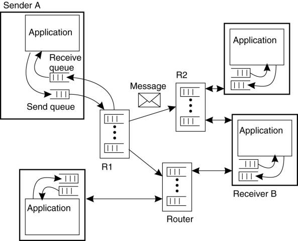
Relays can thus generally
help build scalable message-queuing systems. However, as queuing networks grow,
it is clear that the manual configuration of networks will rapidly become
completely unmanageable. The only solution is to adopt dynamic routing schemes
as is done for computer networks. In that respect, it is somewhat surprising
that such solutions are not yet integrated into some of the popular
message-queuing systems.
[Page 149]
Another reason why relays
are used is that they allow for secondary processing of messages. For example,
messages may need to be logged for reasons of security or fault tolerance. A
special form of relay that we discuss in the next section is one that acts as a
gateway, transforming messages into a format that can be understood by the
receiver.
Finally, relays can be used
for multicasting purposes. In that case, an incoming message is simply put into
each send queue.
Message Brokers
An important application
area of message-queuing systems is integrating existing and new applications
into a single, coherent distributed information system. Integration requires that
applications can understand the messages they receive. In practice, this
requires the sender to have its outgoing messages in the same format as that of
the receiver.
The problem with this
approach is that each time an application is added to the system that requires
a separate message format, each potential receiver will have to be adjusted in
order to produce that format.
An alternative is to agree
on a common message format, as is done with traditional network protocols.
Unfortunately, this approach will generally not work for message-queuing
systems. The problem is the level of abstraction at which these systems
operate. A common message format makes sense only if the collection of
processes that make use of that format indeed have enough in common. If the
collection of applications that make up a distributed information system is
highly diverse (which it often is), then the best common format may well be no
more than a sequence of bytes.
[Page 150]
Although a few common
message formats for specific application domains have been defined, the general
approach is to learn to live with different formats, and try to provide the
means to make conversions as simple as possible. In message-queuing systems,
conversions are handled by special nodes in a queuing network, known as message
brokers. A message broker acts as an application-level gateway in a
message-queuing system. Its main purpose is to convert incoming messages so
that they can be understood by the destination application. Note that to a message-queuing
system, a message broker is just another application, as shown in Fig. 4-21. In
other words, a message broker is generally not considered to be an integral
part of the queuing system.
Figure 4-21. The general
organization of a message broker in a message-queuing system.
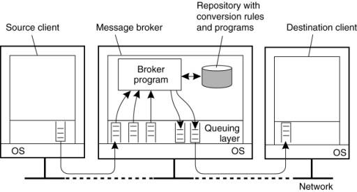
A message broker can be as
simple as a reformatter for messages. For example, assume an incoming message
contains a table from a database, in which records are separated by a special
end-of-record delimiter and fields within a record have a known, fixed length.
If the destination application expects a different delimiter between records,
and also expects that fields have variable lengths, a message broker can be
used to convert messages to the format expected by the destination.
In a more advanced setting,
a message broker may act as an application-level gateway, such as one that
handles the conversion between two different database applications. In such
cases, frequently it cannot be guaranteed that all information contained in the
incoming message can actually be transformed into something appropriate for the
outgoing message.
[Page 151]
However, more common is the
use of a message broker for advanced enterprise application integration (EAI)
as we discussed in Chap. 1. In this case, rather than (only) converting
messages, a broker is responsible for matching applications based on the
messages that are being exchanged. In such a model, called publish/subscribe,
applications send messages in the form of publishing. In particular, they may
publish a message on topic X, which is then sent to the broker. Applications
that have stated their interest in messages on topic X, that is, who have
subscribed to those messages, will then receive these messages from the broker.
More advanced forms of mediation are also possible, but we will defer further
discussion until Chap. 13.
At the heart of a message
broker lies a repository of rules and programs that can transform a message of
type T1 to one of type T2. The problem is defining the rules and developing the
programs. Most message broker products come with sophisticated development
tools, but the bottom line is still that the repository needs to be filled by
experts. Here we see a perfect example where commercial products are often misleadingly
said to provide "intelligence," where, in fact, the only intelligence
is to be found in the heads of those experts.
A Note on Message-Queuing Systems
Considering what we have
said about message-queuing systems, it would appear that they have long existed
in the form of implementations for e-mail services. E-mail systems are
generally implemented through a collection of mail servers that store and
forward messages on behalf of the users on hosts directly connected to the
server. Routing is generally left out, as e-mail systems can make direct use of
the underlying transport services. For example, in the mail protocol for the
Internet, SMTP (Postel, 1982), a message is transferred by setting up a direct
TCP connection to the destination mail server.
What makes e-mail systems
special compared to message-queuing systems is that they are primarily aimed at
providing direct support for end users. This explains, for example, why a
number of groupware applications are based directly on an e-mail system (Khoshafian
and Buckiewicz 1995). In addition, e-mail systems may have very specific
requirements such as automatic message filtering, support for advanced
messaging databases (e.g., to easily retrieve previously stored messages), and
so on.
General message-queuing
systems are not aimed at supporting only end users. An important issue is that
they are set up to enable persistent communication between processes,
regardless of whether a process is running a user application, handling access
to a database, performing computations, and so on. This approach leads to a
different set of requirements for message-queuing systems than pure email
systems. For example, e-mail systems generally need not provide guaranteed
message delivery, message priorities, logging facilities, efficient
multicasting, load balancing, fault tolerance, and so on for general usage.
[Page 152]
General-purpose
message-queuing systems, therefore, have a wide range of applications,
including e-mail, workflow, groupware, and batch processing. However, as we
have stated before, the most important application area is the integration of a
(possibly widely-dispersed) collection of databases and applications into a
federated information system (Hohpe and Woolf, 2004). For example, a query
expanding several databases may need to be split into subqueries that are
forwarded to individual databases. Message-queuing systems assist by providing
the basic means to package each subquery into a message and routing it to the
appropriate database. Other communication facilities we have discussed in this
chapter are far less appropriate.
4.3.3. Example: IBM's WebSphere Message-Queuing System
To help understand how
message-queuing systems work in practice, let us take a look at one specific
system, namely the message-queuing system that is part of IBM's WebSphere
product. Formerly known as MQSeries, it is now referred to as WebSphere MQ.
There is a wealth of documentation on Web-Sphere MQ, and in the following we
can only resort to the basic principles. Many architectural details concerning
message-queuing networks can be found in IBM (2005b, 2005d). Programming
message-queuing networks is not something that can be learned on a Sunday
afternoon, and MQ's programming guide (IBM, 2005a) is a good example showing
that going from principles to practice may require substantial effort.
Overview
The basic architecture of an
MQ queuing network is quite straightforward, and is shown in Fig. 4-22. All
queues are managed by queue managers. A queue manager is responsible for
removing messages from its send queues, and forwarding those to other queue
managers. Likewise, a queue manager is responsible for handling incoming
messages by picking them up from the underlying network and subsequently
storing each message in the appropriate input queue. To give an impression of
what messaging can mean: a message has a maximum default size of 4 MB, but this
can be increased up to 100 MB. A queue is normally restricted to 2 GB of data,
but depending on the underlying operating system, this maximum can be easily
set higher.
Figure 4-22. General
organization of IBM's message-queuing system.
(This item is displayed on
page 153 in the print version)
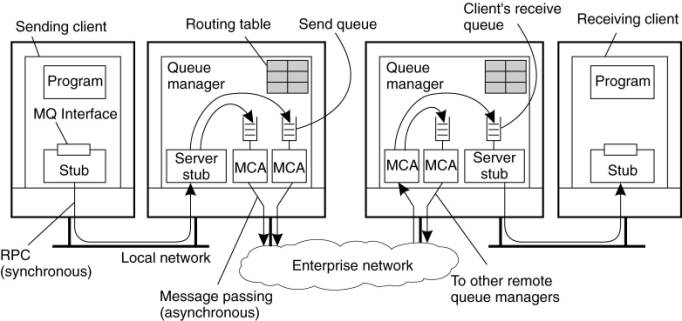
Queue managers are pairwise
connected through message channels, which are an abstraction of transport-level
connections. A message channel is a unidirectional, reliable connection between
a sending and a receiving queue manager, through which queued messages are
transported. For example, an Internet-based message channel is implemented as a
TCP connection. Each of the two ends of a message channel is managed by a
message channel agent (MCA). A sending MCA is basically doing nothing else than
checking send queues for a message, wrapping it into a transport-level packet,
and sending it along the connection to its associated receiving MCA. Likewise,
the basic task of a receiving MCA is listening for an incoming packet,
unwrapping it, and subsequently storing the unwrapped message into the
appropriate queue.
[Page 153]
Queue managers can be linked
into the same process as the application for which it manages the queues. In
that case, the queues are hidden from the application behind a standard
interface, but effectively can be directly manipulated by the application. An
alternative organization is one in which queue managers and applications run on
separate machines. In that case, the application is offered the same interface
as when the queue manager is colocated on the same machine. However, the
interface is implemented as a proxy that communicates with the queue manager
using traditional RPC-based synchronous communication. In this way, MQ
basically retains the model that only queues local to an application can be
accessed.
Channels
An important component of MQ
is formed by the message channels. Each message channel has exactly one
associated send queue from which it fetches the messages it should transfer to
the other end. Transfer along the channel can take place only if both its
sending and receiving MCA are up and running. Apart from starting both MCAs
manually, there are several alternative ways to start a channel, some of which
we discuss next.
[Page 154]
One alternative is to have
an application directly start its end of a channel by activating the sending or
receiving MCA. However, from a transparency point of view, this is not a very
attractive alternative. A better approach to start a sending MCA is to
configure the channel's send queue to set off a trigger when a message is first
put into the queue. That trigger is associated with a handler to start the
sending MCA so that it can remove messages from the send queue.
Another alternative is to
start an MCA over the network. In particular, if one side of a channel is
already active, it can send a control message requesting that the other MCA to
be started. Such a control message is sent to a daemon listening to a
well-known address on the same machine as where the other MCA is to be started.
Channels are stopped
automatically after a specified time has expired during which no more messages
were dropped into the send queue.
Each MCA has a set of
associated attributes that determine the overall behavior of a channel. Some of
the attributes are listed in Fig. 4-23. Attribute values of the sending and
receiving MCA should be compatible and perhaps negotiated first before a
channel can be set up. For example, both MCAs should obviously support the same
transport protocol. An example of a nonnegotiable attribute is whether or not messages
are to be delivered in the same order as they are put into the send queue. If
one MCA wants FIFO delivery, the other must comply. An example of a negotiable
attribute value is the maximum message length, which will simply be chosen as
the minimum value specified by either MCA.
Figure 4-23. Some attributes
associated with message channel agents.
|
Attribute |
Description |
|
Transport type |
Determines the transport
protocol to be used |
|
FIFO delivery |
Indicates that messages are
to be delivered in the order they are sent |
|
Message length |
Maximum length of a single
message |
|
Setup retry count |
Specifies maximum number
of retries to start up the remote MCA |
|
Delivery retries |
Maximum times MCA will try
to put received message into queue |
Message Transfer
To transfer a message from
one queue manager to another (possibly remote) queue manager, it is necessary
that each message carries its destination address, for which a transmission
header is used. An address in MQ consists of two parts. The first part consists
of the name of the queue manager to which the message is to be delivered. The
second part is the name of the destination queue resorting under that manager
to which the message is to be appended.
Besides the destination
address, it is also necessary to specify the route that a message should
follow. Route specification is done by providing the name of the local send
queue to which a message is to be appended. Thus it is not necessary to provide
the full route in a message. Recall that each message channel has exactly one
send queue. By telling to which send queue a message is to be appended, we
efectively specify to which queue manager a message is to be forwarded.
[Page 155]
In most cases, routes are
explicitly stored inside a queue manager in a routing table. An entry in a
routing table is a pair (destQM, sendQ), where destQM is the name of the
destination queue manager, and sendQ is the name of the local send queue to
which a message for that queue manager should be appended. (A routing table
entry is called an alias in MQ.)
It is possible that a
message needs to be transferred across multiple queue managers before reaching
its destination. Whenever such an intermediate queue manager receives the
message, it simply extracts the name of the destination queue manager from the
message header, and does a routing-table look-up to find the local send queue
to which the message should be appended.
It is important to realize
that each queue manager has a systemwide unique name that is effectively used
as an identifier for that queue manager. The problem with using these names is
that replacing a queue manager, or changing its name, will affect all
applications that send messages to it. Problems can be alleviated by using a
local alias for queue manager names. An alias defined within a queue manager M1
is another name for a queue manager M2, but which is available only to
applications interfacing to M1. An alias allows the use of the same (logical)
name for a queue, even if the queue manager of that queue changes. Changing the
name of a queue manager requires that we change its alias in all queue
managers. However, applications can be left unaffected.
[Page 156]
The principle of using routing
tables and aliases is shown in Fig. 4-24. For example, an application linked to
queue manager QMA can refer to a remote queue manager using the local alias
LA1. The queue manager will first look up the actual destination in the alias
table to find it is queue manager QMC. The route to QMC is found in the routing
table, which states that messages for QMC should be appended to the outgoing
queue SQ1, which is used to transfer messages to queue manager QMB. The latter
will use its routing table to forward the message to QMC.
Figure 4-24. The general
organization of an MQ queuing network using routing tables and aliases.
(This item is displayed on
page 155 in the print version)

Following this approach of routing
and aliasing leads to a programming interface that, fundamentally, is
relatively simple, called the Message Queue Interface (MQI). The most important
primitives of MQI are summarized in Fig. 4-25.
Figure 4-25. Primitives
available in the message-queuing interface.
|
Primitive |
Description |
|
MQopen |
Open a (possibly remote)
queue |
|
MQclose |
Close a queue |
|
MQput |
Put a message into an
opened queue |
|
MQget |
Get a message from a
(local) queue |
To put messages into a queue,
an application calls the MQopen primitive, specifying a destination queue in a
specific queue manager. The queue manager can be named using the
locally-available alias. Whether the destination queue is actually remote or
not is completely transparent to the application. MQopen should also be called
if the application wants to get messages from its local queue. Only local
queues can be opened for reading incoming messages. When an application is
finished with accessing a queue, it should close it by calling MQclose.
Messages can be written to,
or read from, a queue using MQput and MQget, respectively. In principle,
messages are removed from a queue on a priority basis. Messages with the same priority
are removed on a first-in, first-out basis, that is, the longest pending
message is removed first. It is also possible to request for specific messages.
Finally, MQ provides facilities to signal applications when messages have
arrived, thus avoiding that an application will continuously have to poll a
message queue for incoming messages.
Managing Overlay Networks
From the description so far,
it should be clear that an important part of managing MQ systems is connecting
the various queue managers into a consistent overlay network. Moreover, this
network needs to be maintained over time. For small networks, this maintenance
will not require much more than average administrative work, but matters become
complicated when message queuing is used to integrate and disintegrate large
existing systems.
[Page 157]
A major issue with MQ is
that overlay networks need to be manually administrated. This administration
not only involves creating channels between queue managers, but also filling in
the routing tables. Obviously, this can grow into a nightmare. Unfortunately,
management support for MQ systems is advanced only in the sense that an
administrator can set virtually every possible attribute, and tweak any
thinkable configuration. However, the bottom line is that channels and routing
tables need to be manually maintained.
At the heart of overlay
management is the channel control function component, which logically sits
between message channel agents. This component allows an operator to monitor
exactly what is going on at two end points of a channel. In addition, it is
used to create channels and routing tables, but also to manage the queue
managers that host the message channel agents. In a way, this approach to
overlay management strongly resembles the management of cluster servers where a
single administration server is used. In the latter case, the server
essentially offers only a remote shell to each machine in the cluster, along
with a few collective operations to handle groups of machines. The good news
about distributed-systems management is that it offers lots of opportunities if
you are looking for an area to explore new solutions to serious problems.
4.4. Stream-Oriented Communication
Communication as discussed
so far has concentrated on exchanging more-or-less independent and complete
units of information. Examples include a request for invoking a procedure, the
reply to such a request, and messages exchanged between applications as in
message-queuing systems. The characteristic feature of this type of
communication is that it does not matter at what particular point in time
communication takes place. Although a system may perform too slow or too fast,
timing has no effect on correctness.
There are also forms of
communication in which timing plays a crucial role. Consider, for example, an
audio stream built up as a sequence of 16-bit samples, each representing the
amplitude of the sound wave as is done through Pulse Code Modulation (PCM).
Also assume that the audio stream represents CD quality, meaning that the
original sound wave has been sampled at a frequency of 44,100 Hz. To reproduce
the original sound, it is essential that the samples in the audio stream are
played out in the order they appear in the stream, but also at intervals of
exactly 1/44,100 sec. Playing out at a different rate will produce an incorrect
version of the original sound.
The question that we address
in this section is which facilities a distributed system should offer to
exchange time-dependent information such as audio and video streams. Various
network protocols that deal with stream-oriented communication are discussed in
Halsall (2001). Steinmetz and Nahrstedt (2004) provide an overall introduction
to multimedia issues, part of which forms stream-oriented communication. Query
processing on data streams is discussed in Babcock et al. (2002).
[Page 158]
4.4.1. Support for Continuous Media
Support for the exchange of
time-dependent information is often formulated as support for continuous media.
A medium refers to the means by which information is conveyed. These means
include storage and transmission media, presentation media such as a monitor,
and so on. An important type of medium is the way that information is
represented. In other words, how is information encoded in a computer system?
Different representations are used for different types of information. For
example, text is generally encoded as ASCII or Unicode. Images can be
represented in different formats such as GIF or JPEG. Audio streams can be
encoded in a computer system by, for example, taking 16-bit samples using PCM.
In continuous
(representation) media, the temporal relationships between different data items
are fundamental to correctly interpreting what the data actually means. We
already gave an example of reproducing a sound wave by playing out an audio
stream. As another example, consider motion. Motion can be represented by a
series of images in which successive images must be displayed at a uniform
spacing T in time, typically 30–40 msec per image. Correct reproduction
requires not only showing the stills in the correct order, but also at a
constant frequency of 1/T images per second.
In contrast to continuous
media, discrete (representation) media, is characterized by the fact that
temporal relationships between data items are not fundamental to correctly
interpreting the data. Typical examples of discrete media include
representations of text and still images, but also object code or executable
files.
Data Stream
To capture the exchange of time-dependent
information, distributed systems generally provide support for data streams. A
data stream is nothing but a sequence of data units. Data streams can be
applied to discrete as well as continuous media. For example, UNIX pipes or
TCP/IP connections are typical examples of (byte-oriented) discrete data
streams. Playing an audio file typically requires setting up a continuous data
stream between the file and the audio device.
Timing is crucial to
continuous data streams. To capture timing aspects, a distinction is often made
between different transmission modes. In asynchronous transmission mode the
data items in a stream are transmitted one after the other, but there are no
further timing constraints on when transmission of items should take place.
This is typically the case for discrete data streams. For example, a file can
be transferred as a data stream, but it is mostly irrelevant exactly when the
transfer of each item completes.
[Page 159]
In synchronous transmission
mode, there is a maximum end-to-end delay defined for each unit in a data
stream. Whether a data unit is transferred much faster than the maximum
tolerated delay is not important. For example, a sensor may sample temperature
at a certain rate and pass it through a network to an operator. In that case,
it may be important that the end-to-end propagation time through the network is
guaranteed to be lower than the time interval between taking samples, but it
cannot do any harm if samples are propagated much faster than necessary.
Finally, in isochronous
transmission mode, it is necessary that data units are transferred on time.
This means that data transfer is subject to a maximum and minimum end-to-end
delay, also referred to as bounded (delay) jitter. Isochronous transmission mode
is particularly interesting for distributed multimedia systems, as it plays a
crucial role in representing audio and video. In this chapter, we consider only
continuous data streams using isochronous transmission, which we will refer to
simply as streams.
Streams can be simple or
complex. A simple stream consists of only a single sequence of data, whereas a
complex stream consists of several related simple streams, called substreams.
The relation between the substreams in a complex stream is often also time
dependent. For example, stereo audio can be transmitted by means of a complex
stream consisting of two substreams, each used for a single audio channel. It
is important, however, that those two substreams are continuously synchronized.
In other words, data units from each stream are to be communicated pairwise to
ensure the effect of stereo. Another example of a complex stream is one for
transmitting a movie. Such a stream could consist of a single video stream,
along with two streams for transmitting the sound of the movie in stereo. A
fourth stream might contain subtitles for the deaf, or a translation into a
different language than the audio. Again, synchronization of the substreams is
important. If synchronization fails, reproduction of the movie fails. We return
to stream synchronization below.
From a distributed systems
perspective, we can distinguish several elements that are needed for supporting
streams. For simplicity, we concentrate on streaming stored data, as opposed to
streaming live data. In the latter case, data is captured in real time and sent
over the network to recipients. The main difference between the two is that
streaming live data leaves less opportunities for tuning a stream. Following Wu
et al. (2001), we can then sketch a general client-server architecture for
supporting continuous multimedia streams as shown in Fig. 4-26.
Figure 4-26. A general
architecture for streaming stored multimedia data over a network.
(This item is displayed on
page 160 in the print version)
[
This general architecture
reveals a number of important issues that need to be dealt with. In the first
place, the multimedia data, notably video and to a lesser extent audio, will
need to be compressed substantially in order to reduce the required storage and
especially the network capacity. More important from the perspective of
communication are controlling the quality of the transmission and
synchronization issues. We discuss these issues next.
[Page 160]
4.4.2. Streams and Quality of Service
Timing (and other
nonfunctional) requirements are generally expressed as Quality of Service (QoS)
requirements. These requirements describe what is needed from the underlying
distributed system and network to ensure that, for example, the temporal
relationships in a stream can be preserved. QoS for continuous data streams
mainly concerns timeliness, volume, and reliability. In this section we take a
closer look at QoS and its relation to setting up a stream.
Much has been said about how
to specify required QoS (see, e.g., Jin and Nahrstedt, 2004). From an
application's perspective, in many cases it boils down to specifying a few
important properties (Halsall, 2001):
- The required bit rate at which data should be
transported.
- The maximum delay until a session has been set
up (i.e., when an application can start sending data).
- The maximum end-to-end delay (i.e., how long it
will take until a data unit makes it to a recipient).
- The maximum delay variance, or jitter.
- The maximum round-trip delay.
It should be noted that many
refinements can be made to these specifications, as explained, for example, by
Steinmetz and Nahrstadt (2004). However, when dealing with stream-oriented
communication that is based on the Internet protocol stack, we simply have to
live with the fact that the basis of communication is formed by an extremely
simple, best-effort datagram service: IP. When the going gets tough, as may
easily be the case in the Internet, the specification of IP allows a protocol
implementation to drop packets whenever it sees fit. Many, if not all
distributed systems that support stream-oriented communication, are currently
built on top of the Internet protocol stack. So much for QoS specifications.
(Actually, IP does provide some QoS support, but it is rarely implemented.)
[Page 161]
Enforcing QoS
Given that the underlying
system offers only a best-effort delivery service, a distributed system can try
to conceal as much as possible of the lack of quality of service. Fortunately,
there are several mechanisms that it can deploy.
First, the situation is not
really so bad as sketched so far. For example, the Internet provides a means
for differentiating classes of data by means of its differentiated services. A
sending host can essentially mark outgoing packets as belonging to one of
several classes, including an expedited forwarding class that essentially
specifies that a packet should be forwarded by the current router with absolute
priority (Davie et al., 2002). In addition, there is also an assured forwarding
class, by which traffic is divided into four subclasses, along with three ways
to drop packets if the network gets congested. Assured forwarding therefore
effectively defines a range of priorities that can be assigned to packets, and
as such allows applications to differentiate time-sensitive packets from
noncritical ones.
Besides these network-level
solutions, a distributed system can also help in getting data across to
receivers. Although there are generally not many tools available, one that is
particularly useful is to use buffers to reduce jitter. The principle is
simple, as shown in Fig. 4-27. Assuming that packets are delayed with a certain
variance when transmitted over the network, the receiver simply stores them in
a buffer for a maximum amount of time. This will allow the receiver to pass
packets to the application at a regular rate, knowing that there will always be
enough packets entering the buffer to be played back at that rate.
Figure 4-27. Using a buffer
to reduce jitter.

Of course, things may go
wrong, as is illustrated by packet #8 in Fig. 4-27. The size of the receiver's
buffer corresponds to 9 seconds of packets to pass to the application.
Unfortunately, packet #8 took 11 seconds to reach the receiver, at which time
the buffer will have been completely emptied. The result is a gap in the
playback at the application. The only solution is to increase the buffer size.
The obvious drawback is that the delay at which the receiving application can
start playing back the data contained in the packets increases as well.
[Page 162]
Other techniques can be used
as well. Realizing that we are dealing with an underlying best-effort service also
means that packets may be lost. To compensate for this loss in quality of
service, we need to apply error correction techniques (Perkins et al., 1998;
and Wah et al., 2000). Requesting the sender to retransmit a missing packet is
generally out of the question, so that forward error correction (FEC) needs to
be applied. A well-known technique is to encode the outgoing packets in such a
way that any k out of n received packets is enough to reconstruct k correct
packets.
One problem that may occur
is that a single packet contains multiple audio and video frames. As a
consequence, when a packet is lost, the receiver may actually perceive a large
gap when playing out frames. This effect can be somewhat circumvented by
interleaving frames, as shown in Fig. 4-28. In this way, when a packet is lost,
the resulting gap in successive frames is distributed over time. Note, however,
that this approach does require a larger receive buffer in comparison to
noninterleaving, and thus imposes a higher start delay for the receiving
application. For example, when considering Fig. 4-28(b), to play the first four
frames, the receiver will need to have four packets delivered, instead of only
one packet in comparison to noninterleaved transmission.
Figure 4-28. The effect of packet
loss in (a) noninterleaved transmission and (b) interleaved transmission.

[Page 163]
4.4.3. Stream Synchronization
An important issue in
multimedia systems is that different streams, possibly in the form of a complex
stream, are mutually synchronized. Synchronization of streams deals with
maintaining temporal relations between streams. Two types of synchronization
occur.
The simplest form of
synchronization is that between a discrete data stream and a continuous data
stream. Consider, for example, a slide show on the Web that has been enhanced
with audio. Each slide is transferred from the server to the client in the form
of a discrete data stream. At the same time, the client should play out a
specific (part of an) audio stream that matches the current slide that is also
fetched from the server. In this case, the audio stream is to be synchronized
with the presentation of slides.
A more demanding type of
synchronization is that between continuous data streams. A daily example is
playing a movie in which the video stream needs to be synchronized with the
audio, commonly referred to as lip synchronization. Another example of
synchronization is playing a stereo audio stream consisting of two substreams,
one for each channel. Proper play out requires that the two substreams are
tightly synchronized: a difference of more than 20 μsec can distort the
stereo effect.
Synchronization takes place
at the level of the data units of which a stream is made up. In other words, we
can synchronize two streams only between data units. The choice of what exactly
a data unit is depends very much on the level of abstraction at which a data
stream is viewed. To make things concrete, consider again a CD-quality
(single-channel) audio stream. At the finest granularity, such a stream appears
as a sequence of 16-bit samples. With a sampling frequency of 44,100 Hz,
synchronization with other audio streams could, in theory, take place
approximately every 23 μsec. For high-quality stereo effects, it turns out
that synchronization at this level is indeed necessary.
However, when we consider
synchronization between an audio stream and a video stream for lip
synchronization, a much coarser granularity can be taken. As we explained,
video frames need to be displayed at a rate of 25 Hz or more. Taking the
widely-used NTSC standard of 29.97 Hz, we could group audio samples into
logical units that last as long as a video frame is displayed (33 msec). With
an audio sampling frequency of 44,100 Hz, an audio data unit can thus be as large
as 1470 samples, or 11,760 bytes (assuming each sample is 16 bits). In
practice, larger units lasting 40 or even 80 msec can be tolerated (Steinmetz,
1996).
Synchronization Mechanisms
Let us now see how
synchronization is actually done. Two issues need to be distinguished: (1) the
basic mechanisms for synchronizing two streams, and (2) the distribution of
those mechanisms in a networked environment.
[Page 164]
Synchronization mechanisms
can be viewed at several different levels of abstraction. At the lowest level,
synchronization is done explicitly by operating on the data units of simple
streams. This principle is shown in Fig. 4-29. In essence, there is a process
that simply executes read and write operations on several simple streams,
ensuring that those operations adhere to specific timing and synchronization
constraints.
Figure 4-29. The principle
of explicit synchronization on the level data units.

For example, consider a
movie that is presented as two input streams. The video stream contains
uncompressed low-quality images of 320x240 pixels, each encoded by a single
byte, leading to video data units of 76,800 bytes each. Assume that images are
to be displayed at 30 Hz, or one image every 33 msec. The audio stream is
assumed to contain audio samples grouped into units of 11760 bytes, each
corresponding to 33 ms of audio, as explained above. If the input process can
handle 2.5 MB/sec, we can achieve lip synchronization by simply alternating
between reading an image and reading a block of audio samples every 33 ms.
The drawback of this
approach is that the application is made completely responsible for
implementing synchronization while it has only low-level facilities available.
A better approach is to offer an application an interface that allows it to
more easily control streams and devices. Returning to our example, assume that
the video display has a control interface that allows it to specify the rate at
which images should be displayed. In addition, the interface offers the
facility to register a user-defined handler that is called each time k new
images have arrived. An analogous interface is offered by the audio device.
With these control interfaces, an application developer can write a simple
monitor program consisting of two handlers, one for each stream, that jointly
check if the video and audio stream are sufficiently synchronized, and if
necessary, adjust the rate at which video or audio units are presented.
This last example is
illustrated in Fig. 4-30, and is typical for many multimedia middleware
systems. In effect, multimedia middleware offers a collection of interfaces for
controlling audio and video streams, including interfaces for controlling
devices such as monitors, cameras, microphones, etc. Each device and stream has
its own high-level interfaces, including interfaces for notifying an
application when some event occurred. The latter are subsequently used to write
handlers for synchronizing streams. Examples of such interfaces are given in
Blair and Stefani (1998).
[Page 165]
Figure 4-30. The principle
of synchronization as supported by high-level interfaces.

[
The distribution of
synchronization mechanisms is another issue that needs to be looked at. First,
the receiving side of a complex stream consisting of substreams that require
synchronization, needs to know exactly what to do. In other words, it must have
a complete synchronization specification locally available. Common practice is
to provide this information implicitly by multiplexing the different streams
into a single stream containing all data units, including those for
synchronization.
This latter approach to
synchronization is followed for MPEG streams. The MPEG (Motion Picture Experts
Group) standards form a collection of algorithms for compressing video and
audio. Several MPEG standards exist. MPEG-2, for example, was originally
designed for compressing broadcast quality video into 4 to 6 Mbps. In MPEG-2,
an unlimited number of continuous and discrete streams can be merged into a
single stream. Each input stream is first turned into a stream of packets that
carry a timestamp based on a 90-kHz system clock. These streams are
subsequently multiplexed into a program stream then consisting of
variable-length packets, but which have in common that they all have the same
time base. The receiving side demultiplexes the stream, again using the
timestamps of each packet as the basic mechanism for interstream
synchronization.
Another important issue is
whether synchronization should take place at the sending or the receiving side.
If the sender handles synchronization, it may be possible to merge streams into
a single stream with a different type of data unit. Consider again a stereo
audio stream consisting of two substreams, one for each channel. One
possibility is to transfer each stream independently to the receiver and let
the latter synchronize the samples pairwise. Obviously, as each substream may
be subject to different delays, synchronization can be extremely difficult. A
better approach is to merge the two substreams at the sender. The resulting
stream consists of data units consisting of pairs of samples, one for each
channel. The receiver now merely has to read in a data unit, and split it into
a left and right sample. Delays for both channels are now identical.
4.5. Multicast Communication
An important topic in
communication in distributed systems is the support for sending data to
multiple receivers, also known as multicast communication. For many years, this
topic has belonged to the domain of network protocols, where numerous proposals
for network-level and transport-level solutions have been implemented and
evaluated (Janic, 2005; and Obraczka, 1998). A major issue in all solutions was
setting up the communication paths for information dissemination. In practice,
this involved a huge management effort, in many cases requiring human
intervention. In addition, as long as there is no convergence of proposals,
ISPs have shown to be reluctant to support multicasting (Diot et al., 2000).
With the advent of peer-to-peer
technology, and notably structured overlay management, it became easier to set
up communication paths. As peer-to-peer solutions are typically deployed at the
application layer, various application-level multicasting techniques have been
introduced. In this section, we will take a brief look at these techniques.
Multicast communication can
also be accomplished in other ways than setting up explicit communication
paths. As we also explore in this section, gossip-based information
dissemination provides simple (yet often less efficient) ways for multicasting.
4.5.1. Application-Level
Multicasting
The basic idea in
application-level multicasting is that nodes organize into an overlay network,
which is then used to disseminate information to its members. An important
observation is that network routers are not involved in group membership. As a
consequence, the connections between nodes in the overlay network may cross
several physical links, and as such, routing messages within the overlay may not
be optimal in comparison to what could have been achieved by network-level
routing.
A crucial design issue is
the construction of the overlay network. In essence, there are two approaches
(El-Sayed, 2003). First, nodes may organize themselves directly into a tree,
meaning that there is a unique (overlay) path between every pair of nodes. An
alternative approach is that nodes organize into a mesh network in which every
node will have multiple neighbors and, in general, there exist multiple paths
between every pair of nodes. The main difference between the two is that the
latter generally provides higher robustness: if a connection breaks (e.g.,
because a node fails), there will still be an opportunity to disseminate
information without having to immediately reorganize the entire overlay
network.
[Page 167]
To make matters concrete,
let us consider a relatively simple scheme for constructing a multicast tree in
Chord, which we described in Chap. 2. This scheme was originally proposed for
Scribe (Castro et al., 2002) which is an application-level multicasting scheme
built on top of Pastry (Rowstron and Druschel, 2001). The latter is also a
DHT-based peer-to-peer system.
Assume a node wants to start
a multicast session. To this end, it simply generates a multicast identifier,
say mid which is just a randomly-chosen 160-bit key. It then looks up
succ(mid), which is the node responsible for that key, and promotes it to
become the root of the multicast tree that will be used to sending data to
interested nodes. In order to join the tree, a node P simply executes the
operation LOOKUP(mid) having the effect that a lookup message with the request
to join the multicast group mid will be routed from P to succ(mid). As we
mentioned before, the routing algorithm itself will be explained in detail in
Chap. 5.
On its way toward the root,
the join request will pass several nodes. Assume it first reaches node Q. If Q
had never seen a join request for mid before, it will become a forwarder for
that group. At that point, P will become a child of Q whereas the latter will
continue to forward the join request to the root. If the next node on the root,
say R is also not yet a forwarder, it will become one and record Q as its child
and continue to send the join request.
On the other hand, if Q (or
R) is already a forwarder for mid, it will also record the previous sender as
its child (i.e., P or Q, respectively), but there will not be a need to send
the join request to the root anymore, as Q (or R) will already be a member of
the multicast tree.
Nodes such as P that have
explicitly requested to join the multicast tree are, by definition, also
forwarders. The result of this scheme is that we construct a multicast tree
across the overlay network with two types of nodes: pure forwarders that act as
helpers, and nodes that are also forwarders, but have explicitly requested to
join the tree. Multicasting is now simple: a node merely sends a multicast
message toward the root of the tree by again executing the LOOKUP(mid)
operation, after which that message can be sent along the tree.
We note that this high-level
description of multicasting in Scribe does not do justice to its original
design. The interested reader is therefore encouraged to take a look at the
details, which can be found in Castro et al. (2002).
Overlay Construction
From the high-level
description given above, it should be clear that although building a tree by
itself is not that difficult once we have organized the nodes into an overlay,
building an efficient tree may be a different story. Note that in our
description so far, the selection of nodes that participate in the tree does
not take into account any performance metrics: it is purely based on the
(logical) routing of messages through the overlay.
[Page 168]
To understand the problem at
hand, take a look at Fig. 4-31 which shows a small set of four nodes that are
organized in a simple overlay network, with node A forming the root of a
multicast tree. The costs for traversing a physical link are also shown. Now,
whenever A multicasts a message to the other nodes, it is seen that this
message will traverse each of the links <B, Rb>, <Ra, Rb>, <Rc,
Rd>, and <D, Rd> twice. The overlay network would have been more
efficient if we had not constructed an overlay link from B to D, but instead
from A to C. Such a configuration would have saved the double traversal across
links <Ra, Rb> and <Rc, Rd>.
Figure 4-31. The relation
between links in an overlay and actual network-level routes.

The quality of an application-level
multicast tree is generally measured by three different metrics: link stress,
stretch, and tree cost. Link stress is defined per link and counts how often a
packet crosses the same link (Chu et al., 2002). A link stress greater than 1 comes
from the fact that although at a logical level a packet may be forwarded along
two different connections, part of those connections may actually correspond to
the same physical link, as we showed in Fig. 4-31.
The stretch or Relative
Delay Penalty (RDP) measures the ratio in the delay between two nodes in the
overlay, and the delay that those two nodes would experience in the underlying
network. For example, in the overlay network, messages from B to C follow the
route B Rb Ra Rc C, having a total cost of 59 units. However,
messages would have been routed in the underlying network along the path B Rb
Rd Rc C, with a total cost of 47 units, leading to a stretch of 1.255.
Obviously, when constructing an overlay network, the goal is to minimize the aggregated
stretch, or similarly, the average RDP measured over all node pairs.
Finally, the tree cost is a
global metric, generally related to minimizing the aggregated link costs. For
example, if the cost of a link is taken to be the delay between its two end
nodes, then optimizing the tree cost boils down to finding a minimal spanning
tree in which the total time for disseminating information to all nodes is
minimal.
[Page 169]
To simplify matters
somewhat, assume that a multicast group has an associated and well-known node
that keeps track of the nodes that have joined the tree. When a new node issues
a join request, it contacts this rendezvous node to obtain a (potentially
partial) list of members. The goal is to select the best member that can operate
as the new node's parent in the tree. Who should it select? There are many
alternatives and different proposals often follow very different solutions.
Consider, for example, a
multicast group with only a single source. In this case, the selection of the
best node is obvious: it should be the source (because in that case we can be
assured that the stretch will be equal to 1). However, in doing so, we would
introduce a star topology with the source in the middle. Although simple, it is
not difficult to imagine the source may easily become overloaded. In other
words, selection of a node will generally be constrained in such a way that
only those nodes may be chosen who have k or less neighbors, with k being a
design parameter. This constraint severely complicates the tree-establishment
algorithm, as a good solution may require that part of the existing tree is
reconfigured.
Tan et al. (2003) provide an
extensive overview and evaluation of various solutions to this problem. As an
illustration, let us take a closer look at one specific family, known as
switch-trees (Helder and Jamin, 2002). The basic idea is simple. Assume we
already have a multicast tree with a single source as root. In this tree, a
node P can switch parents by dropping the link to its current parent in favor
of a link to another node. The only constraints imposed on switching links is
that the new parent can never be a member of the subtree rooted at P (as this
would partition the tree and create a loop), and that the new parent will not
have too many immediate children. The latter is needed to limit the load of
forwarding messages by any single node.
There are different criteria
for deciding to switch parents. A simple one is to optimize the route to the
source, effectively minimizing the delay when a message is to be multicast. To
this end, each node regularly receives information on other nodes (we will
explain one specific way of doing this below). At that point, the node can
evaluate whether another node would be a better parent in terms of delay along
the route to the source, and if so, initiates a switch.
Another criteria could be
whether the delay to the potential other parent is lower than to the current
parent. If every node takes this as a criterion, then the aggregated delays of
the resulting tree should ideally be minimal. In other words, this is an
example of optimizing the cost of the tree as we explained above. However, more
information would be needed to construct such a tree, but as it turns out, this
simple scheme is a reasonable heuristic leading to a good approximation of a
minimal spanning tree.
As an example, consider the
case where a node P receives information on the neighbors of its parent. Note
that the neighbors consist of P's grandparent, along with the other siblings of
P's parent. Node P can then evaluate the delays to each of these nodes and
subsequently choose the one with the lowest delay, say Q, as its new parent. To
that end, it sends a switch request to Q. To prevent loops from being formed
due to concurrent switching requests, a node that has an outstanding switch
request will simply refuse to process any incoming requests. In effect, this
leads to a situation where only completely independent switches can be carried
out simultaneously. Furthermore, P will provide Q with enough information to
allow the latter to conclude that both nodes have the same parent, or that Q is
the grandparent.
[Page 170]
An important problem that we
have not yet addressed is node failure. In the case of switch-trees, a simple
solution is proposed: whenever a node notices that its parent has failed, it
simply attaches itself to the root. At that point, the optimization protocol
can proceed as usual and will eventually place the node at a good point in the
multicast tree. Experiments described in Helder and Jamin (2002) show that the
resulting tree is indeed close to a minimal spanning one.
4.5.2. Gossip-Based Data Dissemination
An increasingly important
technique for disseminating information is to rely on epidemic behavior.
Observing how diseases spread among people, researchers have since long
investigated whether simple techniques could be developed for spreading
information in very large-scale distributed systems. The main goal of these
epidemic protocols is to rapidly propagate information among a large collection
of nodes using only local information. In other words, there is no central
component by which information dissemination is coordinated.
To explain the general principles
of these algorithms, we assume that all updates for a specific data item are
initiated at a single node. In this way, we simply avoid write-write conflicts.
The following presentation is based on the classical paper by Demers et al.
(1987) on epidemic algorithms. A recent overview of epidemic information
dissemination can be found in Eugster at el. (2004).
Information Dissemination
Models
As the name suggests,
epidemic algorithms are based on the theory of epidemics, which studies the
spreading of infectious diseases. In the case of large-scale distributed
systems, instead of spreading diseases, they spread information. Research on
epidemics for distributed systems also aims at a completely different goal:
whereas health organizations will do their utmost best to prevent infectious
diseases from spreading across large groups of people, designers of epidemic
algorithms for distributed systems will try to "infect" all nodes
with new information as fast as possible.
Using the terminology from
epidemics, a node that is part of a distributed system is called infected if it
holds data that it is willing to spread to other nodes. A node that has not yet
seen this data is called susceptible. Finally, an updated node that is not
willing or able to spread its data is said to be removed. Note that we assume
we can distinguish old from new data, for example, because it has been
timestamped or versioned. In this light, nodes are also said to spread updates.
[Page 171]
A popular propagation model
is that of anti-entropy. In this model, a node P picks another node Q at
random, and subsequently exchanges updates with Q. There are three approaches
to exchanging updates:
1. P only pushes its own updates to Q
2. P only pulls in new updates from Q
3. P and Q send updates to each other (i.e., a push-pull
approach)
When it comes to rapidly
spreading updates, only pushing updates turns out to be a bad choice.
Intuitively, this can be understood as follows. First, note that in a pure
push-based approach, updates can be propagated only by infected nodes. However,
if many nodes are infected, the probability of each one selecting a susceptible
node is relatively small. Consequently, chances are that a particular node
remains susceptible for a long period simply because it is not selected by an
infected node.
In contrast, the pull-based
approach works much better when many nodes are infected. In that case,
spreading updates is essentially triggered by susceptible nodes. Chances are
large that such a node will contact an infected one to subsequently pull in the
updates and become infected as well.
It can be shown that if only
a single node is infected, updates will rapidly spread across all nodes using
either form of anti-entropy, although push-pull remains the best strategy
(Jelasity et al., 2005a). Define a round as spanning a period in which every
node will at least once have taken the initiative to exchange updates with a
randomly chosen other node. It can then be shown that the number of rounds to
propagate a single update to all nodes takes O(log (N)) rounds, where N is the
number of nodes in the system. This indicates indeed that propagating updates
is fast, but above all scalable.
One specific variant of this
approach is called rumor spreading, or simply gossiping. It works as follows.
If node P has just been updated for data item x, it contacts an arbitrary other
node Q and tries to push the update to Q. However, it is possible that Q was
already updated by another node. In that case, P may lose interest in spreading
the update any further, say with probability 1/k. In other words, it then
becomes removed.
Gossiping is completely
analogous to real life. When Bob has some hot news to spread around, he may
phone his friend Alice telling her all about it. Alice, like Bob, will be
really excited to spread the gossip to her friends as well. However, she will
become disappointed when phoning a friend, say Chuck, only to hear that the
news has already reached him. Chances are that she will stop phoning other
friends, for what good is it if they already know?
[Page 172]
Gossiping turns out to be an
excellent way of rapidly spreading news. However, it cannot guarantee that all
nodes will actually be updated (Demers et al., 1987). It can be shown that when
there is a large number of nodes that participate in the epidemics, the
fraction s of nodes that will remain ignorant of an update, that is, remain
susceptible, satisfies the equation:
s = e-(k + 1)(1 - s)
Fig. 4-32 shows ln (s) as a function
of k. For example, if k = 4, ln (s)=-4.97, so that s is less than 0.007,
meaning that less than 0.7% of the nodes remain susceptible. Nevertheless,
special measures are needed to guarantee that those nodes will also be updated.
Combining anti-entropy with gossiping will do the trick.
Figure 4-32. The relation
between the fraction s of update-ignorant nodes and the parameter k in pure
gossiping. The graph displays ln(s) as a function of k.
One of the main advantages
of epidemic algorithms is their scalability, due to the fact that the number of
synchronizations between processes is relatively small compared to other
propagation methods. For wide-area systems, Lin and Marzullo (1999) show that
it makes sense to take the actual network topology into account to achieve
better results. In their approach, nodes that are connected to only a few other
nodes are contacted with a relatively high probability. The underlying
assumption is that such nodes form a bridge to other remote parts of the network;
therefore, they should be contacted as soon as possible. This approach is
referred to as directional gossiping and comes in different variants.
This problem touches upon an
important assumption that most epidemic solutions make, namely that a node can
randomly select any other node to gossip with. This implies that, in principle,
the complete set of nodes should be known to each member. In a large system,
this assumption can never hold.
[Page 173]
Fortunately, there is no
need to have such a list. As we explained in Chap. 2, maintaining a partial
view that is more or less continuously updated will organize the collection of
nodes into a random graph. By regularly updating the partial view of each node,
random selection is no longer a problem.
Removing Data
Epidemic algorithms are
extremely good for spreading updates. However, they have a rather strange
side-effect: spreading the deletion of a data item is hard. The essence of the
problem lies in the fact that deletion of a data item destroys all information
on that item. Consequently, when a data item is simply removed from a node,
that node will eventually receive old copies of the data item and interpret
those as updates on something it did not have before.
The trick is to record the
deletion of a data item as just another update, and keep a record of that
deletion. In this way, old copies will not be interpreted as something new, but
merely treated as versions that have been updated by a delete operation. The
recording of a deletion is done by spreading death certificates.
Of course, the problem with
death certificates is that they should eventually be cleaned up, or otherwise
each node will gradually build a huge local database of historical information
on deleted data items that is otherwise not used. Demers et al. (1987) propose
to use what they call dormant death certificates. Each death certificate is
timestamped when it is created. If it can be assumed that updates propagate to
all nodes within a known finite time, then death certificates can be removed
after this maximum propagation time has elapsed.
However, to provide hard
guarantees that deletions are indeed spread to all nodes, only a very few nodes
maintain dormant death certificates that are never thrown away. Assume node P
has such a certificate for data item x. If by any chance an obsolete update for
x reaches P, P will react by simply spreading the death certificate for x
again.
Applications
To finalize this
presentation, let us take a look at some interesting applications of epidemic
protocols. We already mentioned spreading updates, which is perhaps the most
widely-deployed application. Also, in Chap. 2 we discussed how providing
positioning information about nodes can assist in constructing specific
topologies. In the same light, gossiping can be used to discover nodes that
have a few outgoing wide-area links, to subsequently apply directional
gossiping as we mentioned above.
Another interesting
application area is simply collecting, or actually aggregating information (Jelasity
et al., 2005b). Consider the following information exchange. Every node i
initially chooses an arbitrary number, say xi. When node i contacts node j,
they each update their value as:
[Page 174]
xi,xj (xi + xj) /2
Obviously, after this
exchange, both i and j will have the same value. In fact, it is not difficult
to see that eventually all nodes will have the same value, namely the average
of all initial values. Propagation speed is again exponential.
What use does computing the
average have? Consider the situation that all nodes i have set xi to zero,
except for x1, which has set it to 1:
If there N nodes, then
eventually each node will compute the average, which is 1/N. As a consequence,
every node i can estimate the size of the system as being 1/xi. This
information alone can be used to dynamically adjust various system parameters.
For example, the size of the partial view (i.e., the number of neighbors that
each nodes keeps track of) should be dependent on the total number of
participating nodes. Knowing this number will allow a node to dynamically
adjust the size of its partial view. Indeed, this can be viewed as a property
of self-management.
Computing the average may
prove to be difficult when nodes regularly join and leave the system. One
practical solution to this problem is to introduce epochs. Assuming that node 1
is stable, it simply starts a new epoch now and then. When node i sees a new
epoch for the first time, it resets its own variable xi to zero and starts
computing the average again.
Of course, other results can
also be computed. For example, instead of having a fixed node (x1) start the
computation of the average, we can easily pick a random node as follows. Every
node i initially sets xi to a random number from the same interval, say [0,1],
and also stores it permanently as mi. Upon an exchange between nodes i and j,
each change their value to:
xi,xj max (xi,xj)
Each node i for which mi
< xi will lose the competition for being the initiator in starting the
computation of the average. In the end, there will be a single winner. Of
course, although it is easy to conclude that a node has lost, it is much more
difficult to decide that it has won, as it remains uncertain whether all
results have come in. The solution to this problem is to be optimistic: a node
always assumes it is the winner until proven otherwise. At that point, it
simply resets the variable it is using for computing the average to zero. Note
that by now, several different computations (in our example computing a maximum
and computing an average) may be executing concurrently.