Chapter 5. Naming

Names play a very important role in all computer systems. They are used to share resources, to uniquely identify entities, to refer to locations, and more. An important issue with naming is that a name can be resolved to the entity it refers to. Name resolution thus allows a process to access the named entity. To resolve names, it is necessary to implement a naming system. The difference between naming in distributed systems and nondistributed systems lies in the way naming systems are implemented.

In a distributed system, the implementation of a naming system is itself often distributed across multiple machines. How this distribution is done plays a key role in the efficiency and scalability of the naming system. In this chapter, we concentrate on three different, important ways that names are used in distributed systems.

First, after discussing some general issues with respect to naming, we take a closer look at the organization and implementation of human-friendly names. Typical examples of such names include those for file systems and the World Wide Web. Building worldwide, scalable naming systems is a primary concern for these types of names.

Second, names are used to locate entities in a way that is independent of their current location. As it turns out, naming systems for human-friendly names are not particularly suited for supporting this type of tracking down entities. Most names do not even hint at the entity's location. Alternative organizations are needed, such as those being used for mobile telephony where names are locationindependent identifiers, and those for distributed hash tables.

[Page 180]

Finally, humans often prefer to describe entities by means of various characteristics, leading to a situation in which we need to resolve a description by means of attributes to an entity adhering to that description. This type of name resolution is notoriously difficult and we will pay separate attention to it.

5.1. Names, Identifiers, and Addresses

Let us start by taking a closer look at what a name actually is. A name in a distributed system is a string of bits or characters that is used to refer to an entity. An entity in a distributed system can be practically anything. Typical examples include resources such as hosts, printers, disks, and files. Other well-known examples of entities that are often explicitly named are processes, users, mailboxes, newsgroups, Web pages, graphical windows, messages, network connections, and so on.

Entities can be operated on. For example, a resource such as a printer offers an interface containing operations for printing a document, requesting the status of a print job, and the like. Furthermore, an entity such as a network connection may provide operations for sending and receiving data, setting quality-of-service parameters, requesting the status, and so forth.

To operate on an entity, it is necessary to access it, for which we need an access point. An access point is yet another, but special, kind of entity in a distributed system. The name of an access point is called an address. The address of an access point of an entity is also simply called an address of that entity.

An entity can offer more than one access point. As a comparison, a telephone can be viewed as an access point of a person, whereas the telephone number corresponds to an address. Indeed, many people nowadays have several telephone numbers, each number corresponding to a point where they can be reached. In a distributed system, a typical example of an access point is a host running a specific server, with its address formed by the combination of, for example, an IP address and port number (i.e., the server's transport-level address).

An entity may change its access points in the course of time. For example, when a mobile computer moves to another location, it is often assigned a different IP address than the one it had before. Likewise, when a person moves to another city or country, it is often necessary to change telephone numbers as well. In a similar fashion, changing jobs or Internet Service Providers, means changing your e-mail address.

An address is thus just a special kind of name: it refers to an access point of an entity. Because an access point is tightly associated with an entity, it would seem convenient to use the address of an access point as a regular name for the associated entity. Nevertheless, this is hardly ever done as such naming is generally very inflexible and often human unfriendly.

[Page 181]

For example, it is not uncommon to regularly reorganize a distributed system, so that a specific server is now running on a different host than previously. The old machine on which the server used to be running may be reassigned to a completely different server. In other words, an entity may easily change an access point, or an access point may be reassigned to a different entity. If an address is used to refer to an entity, we will have an invalid reference the instant the access point changes or is reassigned to another entity. Therefore, it is much better to let a service be known by a separate name independent of the address of the associated server.

Likewise, if an entity offers more than one access point, it is not clear which address to use as a reference. For instance, many organizations distribute their Web service across several servers. If we would use the addresses of those servers as a reference for the Web service, it is not obvious which address should be chosen as the best one. Again, a much better solution is to have a single name for the Web service independent from the addresses of the different Web servers.

These examples illustrate that a name for an entity that is independent from its addresses is often much easier and more flexible to use. Such a name is called location independent.

In addition to addresses, there are other types of names that deserve special treatment, such as names that are used to uniquely identify an entity. A true identifier is a name that has the following properties (Wieringa and de Jonge, 1995):

1. An identifier refers to at most one entity.

2. Each entity is referred to by at most one identifier.

3. An identifier always refers to the same entity (i.e., it is never reused).

By using identifiers, it becomes much easier to unambiguously refer to an entity. For example, assume two processes each refer to an entity by means of an identifier. To check if the processes are referring to the same entity, it is sufficient to test if the two identifiers are equal. Such a test would not be sufficient if the two processes were using regular, nonunique, nonidentifying names. For example, the name "John Smith" cannot be taken as a unique reference to just a single person.

Likewise, if an address can be reassigned to a different entity, we cannot use an address as an identifier. Consider the use of telephone numbers, which are reasonably stable in the sense that a telephone number for some time refers to the same person or organization. However, using a telephone number as an identifier will not work, as it can be reassigned in the course of time. Consequently, Bob's new bakery may be receiving phone calls for Alice's old antique store for a long time. In this case, it would have been better to use a true identifier for Alice instead of her phone number.

Addresses and identifiers are two important types of names that are each used for very different purposes. In many computer systems, addresses and identifiers are represented in machine-readable form only, that is, in the form of bit strings. For example, an Ethernet address is essentially a random string of 48 bits. Likewise, memory addresses are typically represented as 32-bit or 64-bit strings.

[Page 182]

Another important type of name is that which is tailored to be used by humans, also referred to as human-friendly names. In contrast to addresses and identifiers, a human-friendly name is generally represented as a character string. These names appear in many different forms. For example, files in UNIX systems have character-string names that can be as long as 255 characters, and which are defined entirely by the user. Similarly, DNS names are represented as relatively simple case-insensitive character strings.

Having names, identifiers, and addresses brings us to the central theme of this chapter: how do we resolve names and identifiers to addresses? Before we go into various solutions, it is important to realize that there is often a close relationship between name resolution in distributed systems and message routing. In principle, a naming system maintains a name-to-address binding which in its simplest form is just a table of (name, address) pairs. However, in distributed systems that span large networks and for which many resources need to be named, a centralized table is not going to work.

Instead, what often happens is that a name is decomposed into several parts such as ftp.cs.vu.nl and that name resolution takes place through a recursive look-up of those parts. For example, a client needing to know the address of the FTP server named by ftp.cs.vu.nl would first resolve nl to find the server NS(nl) responsible for names that end with nl, after which the rest of the name is passed to server NS(nl). This server may then resolve the name vu to the server NS(vu.nl) responsible for names that end with vu.nl who can further handle the remaining name ftp.cs. Eventually, this leads to routing the name resolution request as:

NS(.) NS(nl) NS(vu.nl) address of ftp.cs.vu.nl

where NS(.) denotes the server that can return the address of NS(nl), also known as the root server. NS(vu.nl) will return the actual address of the FTP server. It is interesting to note that the boundaries between name resolution and message routing are starting to blur.

In the following sections we will consider three different classes of naming systems. First, we will take a look at how identifiers can be resolved to addresses. In this case, we will also see an example where name resolution is actually indistinguishable from message routing. After that, we consider human-friendly names and descriptive names (i.e., entities that are described by a collection of names).

5.2. Flat Naming

Above, we explained that identifiers are convenient to uniquely represent entities. In many cases, identifiers are simply random bit strings, which we conveniently refer to as unstructured, or flat names. An important property of such a name is that it does not contain any information whatsoever on how to locate the access point of its associated entity. In the following, we will take a look at how flat names can be resolved, or, equivalently, how we can locate an entity when given only its identifier.

[Page 183]

5.2.1. Simple Solutions

We first consider two simple solutions for locating an entity. Both solutions are applicable only to local-area networks. Nevertheless, in that environment, they often do the job well, making their simplicity particularly attractive.

Broadcasting and Multicasting

Consider a distributed system built on a computer network that offers efficient broadcasting facilities. Typically, such facilities are offered by local-area networks in which all machines are connected to a single cable or the logical equivalent thereof. Also, local-area wireless networks fall into this category.

Locating an entity in such an environment is simple: a message containing the identifier of the entity is broadcast to each machine and each machine is requested to check whether it has that entity. Only the machines that can offer an access point for the entity send a reply message containing the address of that access point.

This principle is used in the Internet Address Resolution Protocol (ARP) to find the data-link address of a machine when given only an IP address (Plummer, 1982). In essence, a machine broadcasts a packet on the local network asking who is the owner of a given IP address. When the message arrives at a machine, the receiver checks whether it should listen to the requested IP address. If so, it sends a reply packet containing, for example, its Ethernet address.

Broadcasting becomes inefficient when the network grows. Not only is network bandwidth wasted by request messages, but, more seriously, too many hosts may be interrupted by requests they cannot answer. One possible solution is to switch to multicasting, by which only a restricted group of hosts receives the request. For example, Ethernet networks support data-link level multicasting directly in hardware.

Multicasting can also be used to locate entities in point-to-point networks. For example, the Internet supports network-level multicasting by allowing hosts to join a specific multicast group. Such groups are identified by a multicast address. When a host sends a message to a multicast address, the network layer provides a best-effort service to deliver that message to all group members. Efficient implementations for multicasting in the Internet are discussed in Deering and Cheriton (1990) and Deering et al. (1996).

A multicast address can be used as a general location service for multiple entities. For example, consider an organization where each employee has his or her own mobile computer. When such a computer connects to the locally available network, it is dynamically assigned an IP address. In addition, it joins a specific multicast group. When a process wants to locate computer A, it sends a "where is A?" request to the multicast group. If A is connected, it responds with its current IP address.

[Page 184]

Another way to use a multicast address is to associate it with a replicated entity, and to use multicasting to locate the nearest replica. When sending a request to the multicast address, each replica responds with its current (normal) IP address. A crude way to select the nearest replica is to choose the one whose reply comes in first. We will discuss other ones in later chapters. As it turns out, selecting a nearest replica is generally not that easy.

Forwarding Pointers

Another popular approach to locating mobile entities is to make use of forwarding pointers (Fowler, 1985). The principle is simple: when an entity moves from A to B, it leaves behind in A a reference to its new location at B. The main advantage of this approach is its simplicity: as soon as an entity has been located, for example by using a traditional naming service, a client can look up the current address by following the chain of forwarding pointers.

There are also a number of important drawbacks. First, if no special measures are taken, a chain for a highly mobile entity can become so long that locating that entity is prohibitively expensive. Second, all intermediate locations in a chain will have to maintain their part of the chain of forwarding pointers as long as needed. A third (and related) drawback is the vulnerability to broken links. As soon as any forwarding pointer is lost (for whatever reason) the entity can no longer be reached. An important issue is, therefore, to keep chains relatively short, and to ensure that forwarding pointers are robust.

To better understand how forwarding pointers work, consider their use with respect to remote objects: objects that can be accessed by means of a remote procedure call. Following the approach in SSP chains (Shapiro et al., 1992), each forwarding pointer is implemented as a (client stub, server stub) pair as shown in Fig. 5-1. (We note that in Shapiro's original terminology, a server stub was called a scion, leading to (stub, scion) pairs, which explains its name.) A server stub contains either a local reference to the actual object or a local reference to a remote client stub for that object.

Figure 5-1. The principle of forwarding pointers using (client stub, server stub) pairs.

(This item is displayed on page 185 in the print version)

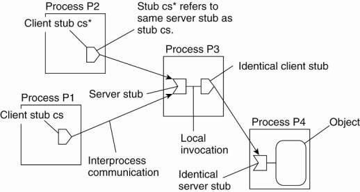
Whenever an object moves from address space A to B, it leaves behind a client stub in its place in A and installs a server stub that refers to it in B. An interesting aspect of this approach is that migration is completely transparent to a client. The only thing the client sees of an object is a client stub. How, and to which location that client stub forwards its invocations, are hidden from the client. Also note that this use of forwarding pointers is not like looking up an address. Instead, a client's request is forwarded along the chain to the actual object.

[Page 185]

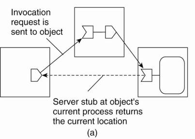
To short-cut a chain of (client stub, server stub) pairs, an object invocation carries the identification of the client stub from where that invocation was initiated. A client-stub identification consists of the client's transport-level address, combined with a locally generated number to identify that stub. When the invocation reaches the object at its current location, a response is sent back to the client stub where the invocation was initiated (often without going back up the chain). The current location is piggybacked with this response, and the client stub adjusts its companion server stub to the one in the object's current location. This principle is shown in Fig. 5-2.

Figure 5-2. Redirecting a forwarding pointer by storing a shortcut in a client stub.

There is a trade-off between sending the response directly to the initiating client stub, or along the reverse path of forwarding pointers. In the former case, communication is faster because fewer processes may need to be passed. On the other hand, only the initiating client stub can be adjusted, whereas sending the response along the reverse path allows adjustment of all intermediate stubs.

[Page 186]

When a server stub is no longer referred to by any client, it can be removed. This by itself is strongly related to distributed garbage collection, a generally far from trivial problem that we will not further discuss here. The interested reader is referred to Abdullahi and Ringwood (1998), Plainfosse and Shapiro (1995), and Veiga and Ferreira (2005).

Now suppose that process P1 in Fig. 5-1 passes its reference to object O to process P2. Reference passing is done by installing a copy p' of client stub p in the address space of process P2. Client stub p' refers to the same server stub as p, so that the forwarding invocation mechanism works the same as before.

Problems arise when a process in a chain of (client stub, server stub) pairs crashes or becomes otherwise unreachable. Several solutions are possible. One possibility, as followed in Emerald (Jul et al., 1988) and in the LII system (Black and Artsy, 1990), is to let the machine where an object was created (called the object's home location), always keep a reference to its current location. That reference is stored and maintained in a fault-tolerant way. When a chain is broken, the object's home location is asked where the object is now. To allow an object's home location to change, a traditional naming service can be used to record the current home location. Such home-based approaches are discussed next.

5.2.2. Home-Based Approaches

The use of broadcasting and forwarding pointers imposes scalability problems. Broadcasting or multicasting is difficult to implement efficiently in largescale networks whereas long chains of forwarding pointers introduce performance problems and are susceptible to broken links.

A popular approach to supporting mobile entities in large-scale networks is to introduce a home location, which keeps track of the current location of an entity. Special techniques may be applied to safeguard against network or process failures. In practice, the home location is often chosen to be the place where an entity was created.

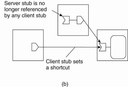
The home-based approach is used as a fall-back mechanism for location services based on forwarding pointers, as discussed above. Another example where the home-based approach is followed is in Mobile IP (Johnson et al., 2004), which we briefly explained in Chap. 3. Each mobile host uses a fixed IP address. All communication to that IP address is initially directed to the mobile host's home agent. This home agent is located on the local-area network corresponding to the network address contained in the mobile host's IP address. In the case of IPv6, it is realized as a network-layer component. Whenever the mobile host moves to another network, it requests a temporary address that it can use for communication. This care-of address is registered at the home agent.

[Page 187]

When the home agent receives a packet for the mobile host, it looks up the host's current location. If the host is on the current local network, the packet is simply forwarded. Otherwise, it is tunneled to the host's current location, that is, wrapped as data in an IP packet and sent to the care-of address. At the same time, the sender of the packet is informed of the host's current location. This principle is shown in Fig. 5-3. Note that the IP address is effectively used as an identifier for the mobile host.

Figure 5-3. The principle of Mobile IP.

Fig. 5-3 also illustrates another drawback of home-based approaches in largescale networks. To communicate with a mobile entity, a client first has to contact the home, which may be at a completely different location than the entity itself. The result is an increase in communication latency.

A drawback of the home-based approach is the use of a fixed home location. For one thing, it must be ensured that the home location always exists. Otherwise, contacting the entity will become impossible. Problems are aggravated when a long-lived entity decides to move permanently to a completely different part of the network than where its home is located. In that case, it would have been better if the home could have moved along with the host.

A solution to this problem is to register the home at a traditional naming service and to let a client first look up the location of the home. Because the home location can be assumed to be relatively stable, that location can be effectively cached after it has been looked up.

[Page 188]

5.2.3. Distributed Hash Tables

Let us now take a closer look at recent developments on how to resolve an identifier to the address of the associated entity. We have already mentioned distributed hash tables a number of times, but have deferred discussion on how they actually work. In this section we correct this situation by first considering the Chord system as an easy-to-explain DHT-based system. In its simplest form, DHT-based systems do not consider network proximity at all. This negligence may easily lead to performance problems. We also discuss solutions for networkaware systems.

General Mechanism

Various DHT-based systems exist, of which a brief overview is given in Balakrishnan et al. (2003). The Chord system (Stoica et al., 2003) is representative for many of them, although there are subtle important differences that influence their complexity in maintenance and lookup protocols. As we explained briefly in Chap. 2, Chord uses an m-bit identifier space to assign randomly-chosen identifiers to nodes as well as keys to specific entities. The latter can be virtually anything: files, processes, etc. The number m of bits is usually 128 or 160, depending on which hash function is used. An entity with key k falls under the jurisdiction of the node with the smallest identifier id k. This node is referred to as the successor of k and denoted as succ(k).

The main issue in DHT-based systems is to efficiently resolve a key k to the address of succ(k). An obvious nonscalable approach is let each node p keep track of the successor succ(p+1) as well as its predecessor pred(p). In that case, whenever a node p receives a request to resolve key k, it will simply forward the request to one of its two neighbors—whichever one is appropriate—unless pred (p) < k p in which case node p should return its own address to the process that initiated the resolution of key k.

Instead of this linear approach toward key lookup, each Chord node maintains a finger table of at most m entries. If FTp denotes the finger table of node p, then

FTp [i ]= succ (p+2i-1)

Put in other words, the i-th entry points to the first node succeeding p by at least 2i-1. Note that these references are actually short-cuts to existing nodes in the identifier space, where the short-cutted distance from node p increases exponentially as the index in the finger table increases. To look up a key k, node p will then immediately forward the request to node q with index j in p's finger table where:

q=FTp [j ] k < FTp [j+1]

(For clarity, we ignore modulo arithmetic.)

[Page 189]

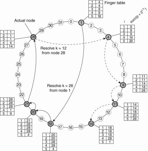
To illustrate this lookup, consider resolving k = 26 from node 1 as shown Fig. 5-4. First, node 1 will look up k = 26 in its finger table to discover that this value is larger than FT 1[5], meaning that the request will be forwarded to node 18 = FT1[5]. Node 18, in turn, will select node 20, as FT18 [2] < k FT18 [3]. Finally, the request is forwarded from node 20 to node 21 and from there to node 28, which is responsible for k = 26. At that point, the address of node 28 is returned to node 1 and the key has been resolved. For similar reasons, when node 28 is requested to resolve the key k = 12, a request will be routed as shown by the dashed line in Fig. 5-4. It can be shown that a lookup will generally require O(log (N)) steps, with N being the number of nodes in the system.

Figure 5-4. Resolving key 26 from node 1 and key 12 from node 28 in a Chord system.

In large distributed systems the collection of participating nodes can be expected to change all the time. Not only will nodes join and leave voluntarily, we also need to consider the case of nodes failing (and thus effectively leaving the system), to later recover again (at which point they join again).

[Page 190]

Joining a DHT-based system such as Chord is relatively simple. Suppose node p wants to join. It simply contacts an arbitrary node in the existing system and requests a lookup for succ(p+1). Once this node has been identified, p can insert itself into the ring. Likewise, leaving can be just as simple. Note that nodes also keep track of their predecessor.

Obviously, the complexity comes from keeping the finger tables up-to-date. Most important is that for every node q, FTq [1] is correct as this entry refers to the next node in the ring, that is, the successor of q+1. In order to achieve this goal, each node q regularly runs a simple procedure that contacts succ(q+1) and requests to return pred(succ(q+1)). If q = pred (succ (q+1)) then q knows its information is consistent with that of its successor. Otherwise, if q's successor has updated its predecessor, then apparently a new node p had entered the system, with q < p succ (q+1), so that q will adjust FTq [1] to p. At that point, it will also check whether p has recorded q as its predecessor. If not, another adjustment of FTq [1] is needed.

In a similar way, to update a finger table, node q simply needs to find the successor for k = q+ 2i-1 for each entry i. Again, this can be done by issuing a request to resolve succ(k). In Chord, such requests are issued regularly by means of a background process.

Likewise, each node q will regularly check whether its predecessor is alive. If the predecessor has failed, the only thing that q can do is record the fact by setting pred(q) to "unknown". On the other hand, when node q is updating its link to the next known node in the ring, and finds that the predecessor of succ(q+1) has been set to "unknown," it will simply notify succ(q+1) that it suspects it to be the predecessor. By and large, these simple procedures ensure that a Chord system is generally consistent, only perhaps with exception of a few nodes. The details can be found in Stoica et al. (2003).

Exploiting Network Proximity

One of the potential problems with systems such as Chord is that requests may be routed erratically across the Internet. For example, assume that node 1 in Fig. 5-4 is placed in Amsterdam, The Netherlands; node 18 in San Diego, California; node 20 in Amsterdam again; and node 21 in San Diego. The result of resolving key 26 will then incur three wide-area message transfers which arguably could have been reduced to at most one. To minimize these pathological cases, designing a DHT-based system requires taking the underlying network into account.

Castro et al. (2002b) distinguish three different ways for making a DHT-based system aware of the underlying network. In the case of topology-based assignment of node identifiers the idea is to assign identifiers such that two nearby nodes will have identifiers that are also close to each other. It is not difficult to imagine that this approach may impose severe problems in the case of relatively simple systems such as Chord. In the case where node identifiers are sampled from a one-dimensional space, mapping a logical ring to the Internet is far from trivial. Moreover, such a mapping can easily expose correlated failures: nodes on the same enterprise network will have identifiers from a relatively small interval. When that network becomes unreachable, we suddenly have a gap in the otherwise uniform distribution of identifiers.

[Page 191]

With proximity routing, nodes maintain a list of alternatives to forward a request to. For example, instead of having only a single successor, each node in Chord could equally well keep track of r successors. In fact, this redundancy can be applied for every entry in a finger table. For node p, FTp [i ] points to the first node in the range [p+2i-1,p+2i-1]. There is no reason why p cannot keep track of r nodes in that range: if needed, each one of them can be used to route a lookup request for a key k > p+2i-1. In that case, when choosing to forward a lookup request, a node can pick one of the r successors that is closest to itself, but also satisfies the constraint that the identifier of the chosen node should be smaller than that of the requested key. An additional advantage of having multiple successors for every table entry is that node failures need not immediately lead to failures of lookups, as multiple routes can be explored.

Finally, in proximity neighbor selection the idea is to optimize routing tables such that the nearest node is selected as neighbor. This selection works only when there are more nodes to choose from. In Chord, this is normally not the case. However, in other protocols such as Pastry (Rowstron and Druschel, 2001), when a node joins it receives information about the current overlay from multiple other nodes. This information is used by the new node to construct a routing table. Obviously, when there are alternative nodes to choose from, proximity neighbor selection will allow the joining node to choose the best one.

Note that it may not be that easy to draw a line between proximity routing and proximity neighbor selection. In fact, when Chord is modified to include r successors for each finger table entry, proximity neighbor selection resorts to identifying the closest r neighbors, which comes very close to proximity routing as we just explained (Dabek at al., 2004b).

Finally, we also note that a distinction can be made between iterative and recursive lookups. In the former case, a node that is requested to look up a key will return the network address of the next node found to the requesting process. The process will then request that next node to take another step in resolving the key. An alternative, and essentially the way that we have explained it so far, is to let a node forward a lookup request to the next node. Both approaches have their advantages and disadvantages, which we explore later in this chapter.

5.2.4. Hierarchical Approaches

In this section, we first discuss a general approach to a hierarchical location scheme, after which a number of optimizations are presented. The approach we present is based on the Globe location service, described in detail in Ballintijn (2003). An overview can be found in van Steen et al. (1998b). This is a generalpurpose location service that is representative of many hierarchical location services proposed for what are called Personal Communication Systems, of which a general overview can be found in Pitoura and Samaras (2001).

[Page 192]

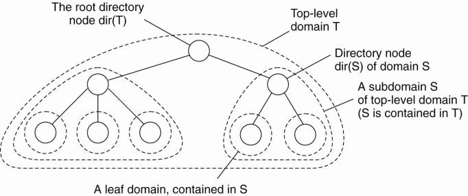
In a hierarchical scheme, a network is divided into a collection of domains. There is a single top-level domain that spans the entire network. Each domain can be subdivided into multiple, smaller subdomains. A lowest-level domain, called a leaf domain, typically corresponds to a local-area network in a computer network or a cell in a mobile telephone network.

Each domain D has an associated directory node dir(D) that keeps track of the entities in that domain. This leads to a tree of directory nodes. The directory node of the top-level domain, called the root (directory) node, knows about all entities. This general organization of a network into domains and directory nodes is illustrated in Fig. 5-5.

Figure 5-5. Hierarchical organization of a location service into domains, each having an associated directory node.

To keep track of the whereabouts of an entity, each entity currently located in a domain D is represented by a location record in the directory node dir(D). A location record for entity E in the directory node N for a leaf domain D contains the entity's current address in that domain. In contrast, the directory node N' for the next higher-level domain D' that contains D, will have a location record for E containing only a pointer to N. Likewise, the parent node of N' will store a location record for E containing only a pointer to N'. Consequently, the root node will have a location record for each entity, where each location record stores a pointer to the directory node of the next lower-level subdomain where that record's associated entity is currently located.

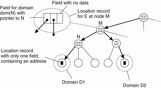
An entity may have multiple addresses, for example if it is replicated. If an entity has an address in leaf domain D1 and D2 respectively, then the directory node of the smallest domain containing both D1 and D2, will have two pointers, one for each subdomain containing an address. This leads to the general organization of the tree as shown in Fig. 5-6.

[Page 193]

Figure 5-6. An example of storing information of an entity having two addresses in different leaf domains.

Let us now consider how a lookup operation proceeds in such a hierarchical location service. As is shown in Fig. 5-7, a client wishing to locate an entity E, issues a lookup request to the directory node of the leaf domain D in which the client resides. If the directory node does not store a location record for the entity, then the entity is currently not located in D. Consequently, the node forwards the request to its parent. Note that the parent node represents a larger domain than its child. If the parent also has no location record for E, the lookup request is forwarded to a next level higher, and so on.

Figure 5-7. Looking up a location in a hierarchically organized location service.

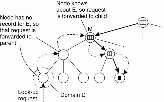
As soon as the request reaches a directory node M that stores a location record for entity E, we know that E is somewhere in the domain dom(M) represented by node M. In Fig. 5-7, M is shown to store a location record containing a pointer to one of its subdomains. The lookup request is then forwarded to the directory node of that subdomain, which in turn forwards it further down the tree, until the request finally reaches a leaf node. The location record stored in the leaf node will contain the address of E in that leaf domain. This address can then be returned to the client that initially requested the lookup to take place.

[Page 194]

An important observation with respect to hierarchical location services is that the lookup operation exploits locality. In principle, the entity is searched in a gradually increasing ring centered around the requesting client. The search area is expanded each time the lookup request is forwarded to a next higher-level directory node. In the worst case, the search continues until the request reaches the root node. Because the root node has a location record for each entity, the request can then simply be forwarded along a downward path of pointers to one of the leaf nodes.

Update operations exploit locality in a similar fashion, as shown in Fig. 5-8. Consider an entity E that has created a replica in leaf domain D for which it needs to insert its address. The insertion is initiated at the leaf node dir(D) of D which immediately forwards the insert request to its parent. The parent will forward the insert request as well, until it reaches a directory node M that already stores a location record for E.

Figure 5-8. (a) An insert request is forwarded to the first node that knows about entity E. (b) A chain of forwarding pointers to the leaf node is created.

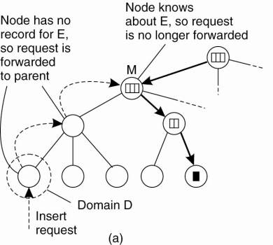
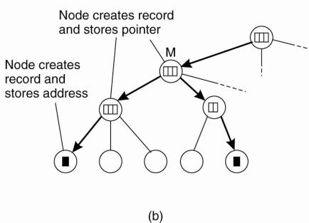
Node M will then store a pointer in the location record for E, referring to the child node from where the insert request was forwarded. At that point, the child node creates a location record for E, containing a pointer to the next lower-level node from where the request came. This process continues until we reach the leaf node from which the insert was initiated. The leaf node, finally, creates a record with the entity's address in the associated leaf domain.

[Page 195]

Inserting an address as just described leads to installing the chain of pointers in a top-down fashion starting at the lowest-level directory node that has a location record for entity E. An alternative is to create a location record before passing the insert request to the parent node. In other words, the chain of pointers is constructed from the bottom up. The advantage of the latter is that an address becomes available for lookups as soon as possible. Consequently, if a parent node is temporarily unreachable, the address can still be looked up within the domain represented by the current node.

A delete operation is analogous to an insert operation. When an address for entity E in leaf domain D needs to be removed, directory node dir(D) is requested to remove that address from its location record for E. If that location record becomes empty, that is, it contains no other addresses for E in D, the record can be removed. In that case, the parent node of dir(D) wants to remove its pointer to dir(D). If the location record for E at the parent now also becomes empty, that record should be removed as well and the next higher-level directory node should be informed. Again, this process continues until a pointer is removed from a location record that remains nonempty afterward or until the root is reached.

5.3. Structured Naming

Flat names are good for machines, but are generally not very convenient for humans to use. As an alternative, naming systems generally support structured names that are composed from simple, human-readable names. Not only file naming, but also host naming on the Internet follow this approach. In this section, we concentrate on structured names and the way that these names are resolved to addresses.

5.3.1. Name Spaces

Names are commonly organized into what is called a name space. Name spaces for structured names can be represented as a labeled, directed graph with two types of nodes. A leaf node represents a named entity and has the property that it has no outgoing edges. A leaf node generally stores information on the entity it is representing—for example, its address—so that a client can access it. Alternatively, it can store the state of that entity, such as in the case of file systems in which a leaf node actually contains the complete file it is representing. We return to the contents of nodes below.

In contrast to a leaf node, a directory node has a number of outgoing edges, each labeled with a name, as shown in Fig. 5-9. Each node in a naming graph is considered as yet another entity in a distributed system, and, in particular, has an associated identifier. A directory node stores a table in which an outgoing edge is represented as a pair (edge label, node identifier). Such a table is called a directory table.

[Page 196]

Figure 5-9. A general naming graph with a single root node.

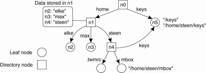
The naming graph shown in Fig. 5-9 has one node, namely n0, which has only outgoing and no incoming edges. Such a node is called the root (node) of the naming graph. Although it is possible for a naming graph to have several root nodes, for simplicity, many naming systems have only one. Each path in a naming graph can be referred to by the sequence of labels corresponding to the edges in that path, such as

N:<label-1, label-2, ..., label-n>

where N refers to the first node in the path. Such a sequence is called a path name. If the first node in a path name is the root of the naming graph, it is called an absolute path name. Otherwise, it is called a relative path name.

It is important to realize that names are always organized in a name space. As a consequence, a name is always defined relative only to a directory node. In this sense, the term "absolute name" is somewhat misleading. Likewise, the difference between global and local names can often be confusing. A global name is a name that denotes the same entity, no matter where that name is used in a system. In other words, a global name is always interpreted with respect to the same directory node. In contrast, a local name is a name whose interpretation depends on where that name is being used. Put differently, a local name is essentially a relative name whose directory in which it is contained is (implicitly) known. We return to these issues later when we discuss name resolution.

This description of a naming graph comes close to what is implemented in many file systems. However, instead of writing the sequence of edge labels to reprepresent a path name, path names in file systems are generally represented as a single string in which the labels are separated by a special separator character, such as a slash ("/"). This character is also used to indicate whether a path name is absolute. For example, in Fig. 5-9, instead of using n0:<home, steen, mbox>, that is, the actual path name, it is common practice to use its string representation /home/steen/mbox. Note also that when there are several paths that lead to the same node, that node can be represented by different path names. For example, node n5 in Fig. 5-9 can be referred to by /home/steen/keys as well as /keys. The string representation of path names can be equally well applied to naming graphs other than those used for only file systems. In Plan 9 (Pike et al., 1995), all resources, such as processes, hosts, I/O devices, and network interfaces, are named in the same fashion as traditional files. This approach is analogous to implementing a single naming graph for all resources in a distributed system.

[Page 197]

There are many different ways to organize a name space. As we mentioned, most name spaces have only a single root node. In many cases, a name space is also strictly hierarchical in the sense that the naming graph is organized as a tree. This means that each node except the root has exactly one incoming edge; the root has no incoming edges. As a consequence, each node also has exactly one associated (absolute) path name.

The naming graph shown in Fig. 5-9 is an example of directed acyclic graph. In such an organization, a node can have more than one incoming edge, but the graph is not permitted to have a cycle. There are also name spaces that do not have this restriction.

To make matters more concrete, consider the way that files in a traditional UNIX file system are named. In a naming graph for UNIX, a directory node represents a file directory, whereas a leaf node represents a file. There is a single root directory, represented in the naming graph by the root node. The implementation of the naming graph is an integral part of the complete implementation of the file system. That implementation consists of a contiguous series of blocks from a logical disk, generally divided into a boot block, a superblock, a series of index nodes (called inodes), and file data blocks. See also Crowley (1997), Silberschatz et al. (2005), and Tanenbaum and Woodhull (2006). This organization is shown in Fig. 5-10.

Figure 5-10. The general organization of the UNIX file system implementation on a logical disk of contiguous disk blocks.

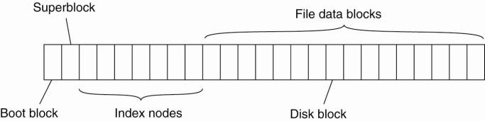
The boot block is a special block of data and instructions that are automatically loaded into main memory when the system is booted. The boot block is used to load the operating system into main memory.

[Page 198]

The superblock contains information on the entire file system, such as its size, which blocks on disk are not yet allocated, which inodes are not yet used, and so on. Inodes are referred to by an index number, starting at number zero, which is reserved for the inode representing the root directory.

Each inode contains information on where the data of its associated file can be found on disk. In addition, an inode contains information on its owner, time of creation and last modification, protection, and the like. Consequently, when given the index number of an inode, it is possible to access its associated file. Each directory is implemented as a file as well. This is also the case for the root directory, which contains a mapping between file names and index numbers of inodes. It is thus seen that the index number of an inode corresponds to a node identifier in the naming graph.

5.3.2. Name Resolution

Name spaces offer a convenient mechanism for storing and retrieving information about entities by means of names. More generally, given a path name, it should be possible to look up any information stored in the node referred to by that name. The process of looking up a name is called name resolution.

To explain how name resolution works, let us consider a path name such as N:<label1, label2, ..., labeln>. Resolution of this name starts at node N of the naming graph, where the name label1 is looked up in the directory table, and which returns the identifier of the node to which label1 refers. Resolution then continues at the identified node by looking up the name label2 in its directory table, and so on. Assuming that the named path actually exists, resolution stops at the last node referred to by labeln, by returning the content of that node.

A name lookup returns the identifier of a node from where the name resolution process continues. In particular, it is necessary to access the directory table of the identified node. Consider again a naming graph for a UNIX file system. As mentioned, a node identifier is implemented as the index number of an inode. Accessing a directory table means that first the inode has to be read to find out where the actual data are stored on disk, and then subsequently to read the data blocks containing the directory table.

Closure Mechanism

Name resolution can take place only if we know how and where to start. In our example, the starting node was given, and we assumed we had access to its directory table. Knowing how and where to start name resolution is generally referred to as a closure mechanism. Essentially, a closure mechanism deals with selecting the initial node in a name space from which name resolution is to start (Radia, 1989). What makes closure mechanisms sometimes hard to understand is that they are necessarily partly implicit and may be very different when comparing them to each other.

[Page 199]

For example, name resolution in the naming graph for a UNIX file system makes use of the fact that the inode of the root directory is the first inode in the logical disk representing the file system. Its actual byte offset is calculated from the values in other fields of the superblock, together with hard-coded information in the operating system itself on the internal organization of the superblock.

To make this point clear, consider the string representation of a file name such as /home/steen/mbox. To resolve this name, it is necessary to already have access to the directory table of the root node of the appropriate naming graph. Being a root node, the node itself cannot have been looked up unless it is implemented as a different node in a another naming graph, say G. But in that case, it would have been necessary to already have access to the root node of G. Consequently, resolving a file name requires that some mechanism has already been implemented by which the resolution process can start.

A completely different example is the use of the string "0031204430784". Many people will not know what to do with these numbers, unless they are told that the sequence is a telephone number. That information is enough to start the resolution process, in particular, by dialing the number. The telephone system subsequently does the rest.

As a last example, consider the use of global and local names in distributed systems. A typical example of a local name is an environment variable. For example, in UNIX systems, the variable named HOME is used to refer to the home directory of a user. Each user has its own copy of this variable, which is initialized to the global, systemwide name corresponding to the user's home directory. The closure mechanism associated with environment variables ensures that the name of the variable is properly resolved by looking it up in a user-specific table.

Linking and Mounting

Strongly related to name resolution is the use of aliases. An alias is another name for the same entity. An environment variable is an example of an alias. In terms of naming graphs, there are basically two different ways to implement an alias. The first approach is to simply allow multiple absolute paths names to refer to the same node in a naming graph. This approach is illustrated in Fig. 5-9, in which node n5 can be referred to by two different path names. In UNIX terminology, both path names /keys and /home/steen/keys in Fig. 5-9 are called hard links to node n5.

The second approach is to represent an entity by a leaf node, say N, but instead of storing the address or state of that entity, the node stores an absolute path name. When first resolving an absolute path name that leads to N, name resolution will return the path name stored in N, at which point it can continue with resolving that new path name. 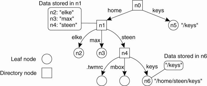This principle corresponds to the use of symbolic links in UNIX file systems, and is illustrated in Fig. 5-11. In this example, the path name /home/steen/keys, which refers to a node containing the absolute path name /keys, is a symbolic link to node n5.

[Page 200]

Figure 5-11. The concept of a symbolic link explained in a naming graph.

Name resolution as described so far takes place completely within a single name space. However, name resolution can also be used to merge different name spaces in a transparent way. Let us first consider a mounted file system. In terms of our naming model, a mounted file system corresponds to letting a directory node store the identifier of a directory node from a different name space, which we refer to as a foreign name space. The directory node storing the node identifier is called a mount point. Accordingly, the directory node in the foreign name space is called a mounting point. Normally, the mounting point is the root of a name space. During name resolution, the mounting point is looked up and resolution proceeds by accessing its directory table.

The principle of mounting can be generalized to other name spaces as well. In particular, what is needed is a directory node that acts as a mount point and stores all the necessary information for identifying and accessing the mounting point in the foreign name space. This approach is followed in many distributed file systems.

Consider a collection of name spaces that is distributed across different machines. In particular, each name space is implemented by a different server, each possibly running on a separate machine. Consequently, if we want to mount a foreign name space NS2 into a name space NS1, it may be necessary to communicate over a network with the server of NS2, as that server may be running on a different machine than the server for NS1. To mount a foreign name space in a distributed system requires at least the following information:

1. The name of an access protocol.

2. The name of the server.

3. The name of the mounting point in the foreign name space.

[Page 201]

Note that each of these names needs to be resolved. The name of an access protocol needs to be resolved to the implementation of a protocol by which communication with the server of the foreign name space can take place. The name of the server needs to be resolved to an address where that server can be reached. As the last part in name resolution, the name of the mounting point needs to be resolved to a node identifier in the foreign name space.

In nondistributed systems, none of the three points may actually be needed. For example, in UNIX, there is no access protocol and no server. Also, the name of the mounting point is not necessary, as it is simply the root directory of the foreign name space.

The name of the mounting point is to be resolved by the server of the foreign name space. However, we also need name spaces and implementations for the access protocol and the server name. One possibility is to represent the three names listed above as a URL.

To make matters concrete, consider a situation in which a user with a laptop computer wants to access files that are stored on a remote file server. The client machine and the file server are both configured with Sun's Network File System (NFS), which we will discuss in detail in Chap. 11. NFS is a distributed file system that comes with a protocol that describes precisely how a client can access a file stored on a (remote) NFS file server. In particular, to allow NFS to work across the Internet, a client can specify exactly which file it wants to access by means of an NFS URL, for example, nfs://flits.cs.vu.nl//home/steen. This URL names a file (which happens to be a directory) called /home/steen on an NFS file server flits.cs.vu.nl, which can be accessed by a client by means of the NFS protocol (Shepler et al., 2003).

The name nfs is a well-known name in the sense that worldwide agreement exists on how to interpret that name. Given that we are dealing with a URL, the name nfs will be resolved to an implementation of the NFS protocol. The server name is resolved to its address using DNS, which is discussed in a later section. As we said, /home/steen is resolved by the server of the foreign name space.

The organization of a file system on the client machine is partly shown in Fig. 5-12. The root directory has a number of user-defined entries, including a subdirectory called /remote. This subdirectory is intended to include mount points for foreign name spaces such as the user's home directory at the Vrije Universiteit. To this end, a directory node named /remote/vu is used to store the URL nfs://flits.cs.vu.nl//home/steen.

Figure 5-12. Mounting remote name spaces through a specific access protocol.

(This item is displayed on page 202 in the print version)

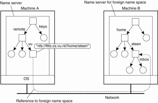
Now consider the name /remote/vu/mbox. This name is resolved by starting in the root directory on the client's machine and continues until the node /remote/vu is reached. The process of name resolution then continues by returning the URL nfs://flits.cs.vu.nl//home/steen, in turn leading the client machine to contact the file server flits.cs.vu.nl by means of the NFS protocol, and to subsequently access directory /home/steen. Name resolution can then be continued by reading the file named mbox in that directory, after which the resolution process stops.

[Page 202]

Distributed systems that allow mounting a remote file system as just described allow a client machine to, for example, execute the following commands:

cd /remote/vu

ls –l

which subsequently lists the files in the directory /home/steen on the remote file server. The beauty of all this is that the user is spared the details of the actual access to the remote server. Ideally, only some loss in performance is noticed compared to accessing locally-available files. In effect, to the client it appears that the name space rooted on the local machine, and the one rooted at /home/steen on the remote machine, form a single name space.

5.3.3. The Implementation of a Name Space

A name space forms the heart of a naming service, that is, a service that allows users and processes to add, remove, and look up names. A naming service is implemented by name servers. If a distributed system is restricted to a localarea network, it is often feasible to implement a naming service by means of only a single name server. However, in large-scale distributed systems with many entities, possibly spread across a large geographical area, it is necessary to distribute the implementation of a name space over multiple name servers.

Name Space Distribution

Name spaces for a large-scale, possibly worldwide distributed system, are usually organized hierarchically. As before, assume such a name space has only a single root node. To effectively implement such a name space, it is convenient to partition it into logical layers. Cheriton and Mann (1989) distinguish the following three layers.

The global layer is formed by highest-level nodes, that is, the root node and other directory nodes logically close to the root, namely its children. Nodes in the global layer are often characterized by their stability, in the sense that directory tables are rarely changed. Such nodes may represent organizations, or groups of organizations, for which names are stored in the name space.

The administrational layer is formed by directory nodes that together are managed within a single organization. A characteristic feature of the directory nodes in the administrational layer is that they represent groups of entities that belong to the same organization or administrational unit. For example, there may be a directory node for each department in an organization, or a directory node from which all hosts can be found. Another directory node may be used as the starting point for naming all users, and so forth. The nodes in the administrational layer are relatively stable, although changes generally occur more frequently than to nodes in the global layer.

Finally, the managerial layer consists of nodes that may typically change regularly. For example, nodes representing hosts in the local network belong to this layer. For the same reason, the layer includes nodes representing shared files such as those for libraries or binaries. Another important class of nodes includes those that represent user-defined directories and files. In contrast to the global and administrational layer, the nodes in the managerial layer are maintained not only by system administrators, but also by individual end users of a distributed system.

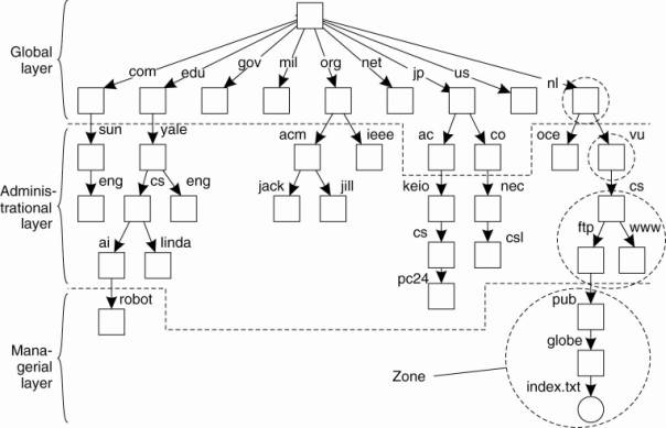
To make matters more concrete, Fig. 5-13 shows an example of the partitioning of part of the DNS name space, including the names of files within an organization that can be accessed through the Internet, for example, Web pages and transferable files. The name space is divided into nonoverlapping parts, called zones in DNS (Mockapetris, 1987). A zone is a part of the name space that is implemented by a separate name server. Some of these zones are illustrated in Fig. 5-13.

Figure 5-13. An example partitioning of the DNS name space, including Internet-accessible files, into three layers.

(This item is displayed on page 204 in the print version)

If we take a look at availability and performance, name servers in each layer have to meet different requirements. High availability is especially critical for name servers in the global layer. If a name server fails, a large part of the name space will be unreachable because name resolution cannot proceed beyond the failing server.

Performance is somewhat subtle. Due to the low rate of change of nodes in the global layer, the results of lookup operations generally remain valid for a long time. Consequently, those results can be effectively cached (i.e., stored locally) by the clients. The next time the same lookup operation is performed, the results can be retrieved from the client's cache instead of letting the name server return the results. As a result, name servers in the global layer do not have to respond quickly to a single lookup request. On the other hand, throughput may be important, especially in large-scale systems with millions of users.

[Page 204]

The availability and performance requirements for name servers in the global layer can be met by replicating servers, in combination with client-side caching. As we discuss in Chap. 7, updates in this layer generally do not have to come into effect immediately, making it much easier to keep replicas consistent.

Availability for a name server in the administrational layer is primarily important for clients in the same organization as the name server. If the name server fails, many resources within the organization become unreachable because they cannot be looked up. On the other hand, it may be less important that resources in an organization are temporarily unreachable for users outside that organization.

With respect to performance, name servers in the administrational layer have similar characteristics as those in the global layer. Because changes to nodes do not occur all that often, caching lookup results can be highly effective, making performance less critical. However, in contrast to the global layer, the administrational layer should take care that lookup results are returned within a few milliseconds, either directly from the server or from the client's local cache. Likewise, updates should generally be processed quicker than those of the global layer. For example, it is unacceptable that an account for a new user takes hours to become effective.

[Page 205]

These requirements can often be met by using high-performance machines to run name servers. In addition, client-side caching should be applied, combined with replication for increased overall availability.

Availability requirements for name servers at the managerial level are generally less demanding. In particular, it often suffices to use a single (dedicated) machine to run name servers at the risk of temporary unavailability. However, performance is crucial. Users expect operations to take place immediately. Because updates occur regularly, client-side caching is often less effective, unless special measures are taken, which we discuss in Chap. 7.

A comparison between name servers at different layers is shown in Fig. 5-14. In distributed systems, name servers in the global and administrational layer are the most difficult to implement. Difficulties are caused by replication and caching, which are needed for availability and performance, but which also introduce consistency problems. Some of the problems are aggravated by the fact that caches and replicas are spread across a wide-area network, which introduces long communication delays thereby making synchronization even harder. Replication and caching are discussed extensively in Chap. 7.

Figure 5-14. A comparison between name servers for implementing nodes from a large-scale name space partitioned into a global layer, an administrational layer, and a managerial layer.

Item	Global	Administrational	Managerial
Geographical scale of network	Worldwide	Organization	Department
Total number of nodes	Few	Many	Vast numbers
Responsiveness to lookups	Seconds	Milliseconds	Immediate
Update propagation	Lazy	Immediate	Immediate
Number of replicas	Many	None or few	None
Is client-side caching applied?	Yes	Yes	Sometimes

Implementation of Name Resolution

The distribution of a name space across multiple name servers affects the implementation of name resolution. To explain the implementation of name resolution in large-scale name services, we assume for the moment that name servers are not replicated and that no client-side caches are used. Each client has access to a local name resolver, which is responsible for ensuring that the name resolution process is carried out. Referring to Fig. 5-13, assume the (absolute) path name

[Page 206]

root:<nl, vu, cs, ftp, pub, globe, index.html >

is to be resolved. Using a URL notation, this path name would correspond to ftp://ftp.cs.vu.nl/pub/globe/index.html. There are now two ways to implement name resolution.

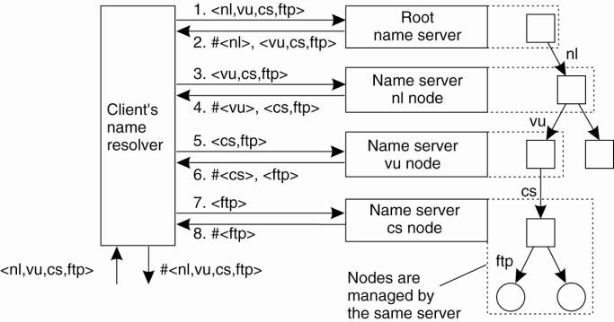
In iterative name resolution, a name resolver hands over the complete name to the root name server. It is assumed that the address where the root server can be contacted is well known. The root server will resolve the path name as far as it can, and return the result to the client. In our example, the root server can resolve only the label nl, for which it will return the address of the associated name server.

At that point, the client passes the remaining path name (i.e., nl:<vu, cs, ftp, pub, globe, index.html >) to that name server. This server can resolve only the label vu, and returns the address of the associated name server, along with the remaining path name vu:<cs, ftp, pub, globe, index.html >.

The client's name resolver will then contact this next name server, which responds by resolving the label cs, and subsequently also ftp, returning the address of the FTP server along with the path name ftp:<pub, globe, index.html >. The client then contacts the FTP server, requesting it to resolve the last part of the original path name. The FTP server will subsequently resolve the labels pub, globe, and index.html, and transfer the requested file (in this case using FTP). 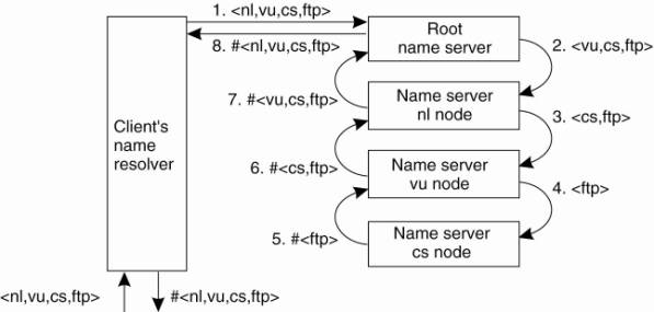This process of iterative name resolution is shown in Fig. 5-15. (The notation #<cs> is used to indicate the address of the server responsible for handling the node referred to by <cs>.)

Figure 5-15. The principle of iterative name resolution.

[Page 207]

In practice, the last step, namely contacting the FTP server and requesting it to transfer the file with path name ftp:<pub, globe, index.html >, is carried out separately by the client process. In other words, the client would normally hand only the path name root:<nl, vu, cs, ftp> to the name resolver, from which it would expect the address where it can contact the FTP server, as is also shown in Fig. 5-15.

An alternative to iterative name resolution is to use recursion during name resolution. Instead of returning each intermediate result back to the client's name resolver, with recursive name resolution, a name server passes the result to the next name server it finds. So, for example, when the root name server finds the address of the name server implementing the node named nl, it requests that name server to resolve the path name nl:<vu, cs, ftp, pub, globe, index.html >. Using recursive name resolution as well, this next server will resolve the complete path and eventually return the file index.html to the root server, which, in turn, will pass that file to the client's name resolver.

Recursive name resolution is shown in Fig. 5-16. As in iterative name resolution, the last resolution step (contacting the FTP server and asking it to transfer the indicated file) is generally carried out as a separate process by the client.

Figure 5-16. The principle of recursive name resolution.

The main drawback of recursive name resolution is that it puts a higher performance demand on each name server. Basically, a name server is required to handle the complete resolution of a path name, although it may do so in cooperation with other name servers. This additional burden is generally so high that name servers in the global layer of a name space support only iterative name resolution.

There are two important advantages to recursive name resolution. The first advantage is that caching results is more effective compared to iterative name resolution. The second advantage is that communication costs may be reduced. To explain these advantages, assume that a client's name resolver will accept path names referring only to nodes in the global or administrational layer of the name space. To resolve that part of a path name that corresponds to nodes in the managerial layer, a client will separately contact the name server returned by its name resolver, as we discussed above.

[Page 208]

Recursive name resolution allows each name server to gradually learn the address of each name server responsible for implementing lower-level nodes. As a result, caching can be effectively used to enhance performance. For example, when the root server is requested to resolve the path name root:<nl, vu, cs, ftp>, it will eventually get the address of the name server implementing the node referred to by that path name. To come to that point, the name server for the nl node has to look up the address of the name server for the vu node, whereas the latter has to look up the address of the name server handling the cs node.

Because changes to nodes in the global and administrational layer do not occur often, the root name server can effectively cache the returned address. Moreover, because the address is also returned, by recursion, to the name server responsible for implementing the vu node and to the one implementing the nl node, it might as well be cached at those servers too.

Likewise, the results of intermediate name lookups can also be returned and cached. For example, the server for the nl node will have to look up the address of the vu node server. That address can be returned to the root server when the nl server returns the result of the original name lookup. A complete overview of the resolution process, and the results that can be cached by each name server is shown in Fig. 5-17.

Figure 5-17. Recursive name resolution of <nl, vu, cs, ftp>. Name servers cache intermediate results for subsequent lookups.

Server for node	Should resolve	Looks up	Passes to child	Receives and caches	Returns to requester
cs	<ftp>	#<ftp>	—	—	#<ftp>
vu	<cs,ftp>	#<cs>	<ftp>	#<ftp>	#<cs> #<cs, ftp>
nl	<vu,cs,ftp>	#<vu>	<cs,ftp>	#<cs> #<cs,ftp>	#<vu> #<vu,cs> #<vu,cs,ftp>
root	<nl,vu,cs,ftp>	#<nl>	<vu,cs,ftp>	#<vu> #<vu,cs> #<vu,cs,ftp>	#<nl> #<nl,vu> #<nl,vu,cs> #<nl,vu,cs,ftp>

The main benefit of this approach is that, eventually, lookup operations can be handled quite efficiently. For example, suppose that another client later requests resolution of the path name root:<nl, vu, cs, flits>. This name is passed to the root, which can immediately forward it to the name server for the cs node, and request it to resolve the remaining path name cs:<flits>.

[Page 209]

With iterative name resolution, caching is necessarily restricted to the client's name resolver. Consequently, if a client A requests the resolution of a name, and another client B later requests that same name to be resolved, name resolution will have to pass through the same name servers as was done for client A. As a compromise, many organizations use a local, intermediate name server that is shared by all clients. This local name server handles all naming requests and caches results. Such an intermediate server is also convenient from a management point of view. For example, only that server needs to know where the root name server is located; other machines do not require this information.

The second advantage of recursive name resolution is that it is often cheaper with respect to communication. Again, consider the resolution of the path name root:<nl, vu, cs, ftp> and assume the client is located in San Francisco. Assuming that the client knows the address of the server for the nl node, with recursive name resolution, communication follows the route from the client's host in San Francisco to the nl server in The Netherlands, shown as R 1 in Fig. 5-18. From there on, communication is subsequently needed between the nl server and the name server of the Vrije Universiteit on the university campus in Amsterdam, The Netherlands. This communication is shown as R 2. Finally, communication is needed between the vu server and the name server in the Computer Science Department, shown as R 3. The route for the reply is the same, but in the opposite direction. Clearly, communication costs are dictated by the message exchange between the client's host and the nl server.

Figure 5-18. The comparison between recursive and iterative name resolution with respect to communication costs.

(This item is displayed on page 210 in the print version)

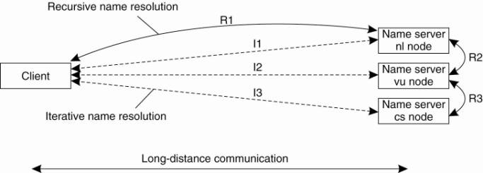
In contrast, with iterative name resolution, the client's host has to communicate separately with the nl server, the vu server, and the cs server, of which the total costs may be roughly three times that of recursive name resolution. The arrows in Fig. 5-18 labeled I 1, I 2, and I 3 show the communication path for iterative name resolution.

5.3.4. Example: The Domain Name System

One of the largest distributed naming services in use today is the Internet Domain Name System (DNS). DNS is primarily used for looking up IP addresses of hosts and mail servers. In the following pages, we concentrate on the organization of the DNS name space, and the information stored in its nodes. Also, we take a closer look at the actual implementation of DNS. More information can be found in Mockapetris (1987) and Albitz and Liu (2001). A recent assessment of DNS, notably concerning whether it still fits the needs of the current Internet, can be found in Levien (2005). From this report, one can draw the somewhat surprising conclusion that even after more than 30 years, DNS gives no indication that it needs to be replaced. We would argue that the main cause lies in the designer's deep understanding of how to keep matters simple. Practice in other fields of distributed systems indicates that not many are gifted with such an understanding.

[Page 210]

The DNS Name Space

The DNS name space is hierarchically organized as a rooted tree. A label is a case-insensitive string made up of alphanumeric characters. A label has a maximum length of 63 characters; the length of a complete path name is restricted to 255 characters. The string representation of a path name consists of listing its labels, starting with the rightmost one, and separating the labels by a dot ("."). The root is represented by a dot. So, for example, the path name root:<nl, vu, cs, flits>, is represented by the string flits.cs.vu.nl., which includes the rightmost dot to indicate the root node. We generally omit this dot for readability.

Because each node in the DNS name space has exactly one incoming edge (with the exception of the root node, which has no incoming edges), the label attached to a node's incoming edge is also used as the name for that node. A subtree is called a domain; a path name to its root node is called a domain name. Note that, just like a path name, a domain name can be either absolute or relative.

The contents of a node is formed by a collection of resource records. There are different types of resource records. The major ones are shown in Fig. 5-19.

Figure 5-19. The most important types of resource records forming the contents of nodes in the DNS name space.

(This item is displayed on page 211 in the print version)

Type of record	Associated entity	Description
SOA	Zone	Holds information on the represented zone
A	Host	Contains an IP address of the host this node represents
MX	Domain	Refers to a mail server tohandle mail addressed to this node
SRV	Domain	Refers to a server handling a specific service
NS	Zone	Refers to a name server that implements the represented zone
CNAME	Node	Symbolic link with the primary name of the represented node
PTR	Host	Contains the canonical name of a host
HINFO	Host	Holds information on the host this node represents
TXT	Any kind	Contains any entity-specific information considered useful

A node in the DNS name space often will represent several entities at the same time. For example, a domain name such as vu.nl is used to represent a domain and a zone. In this case, the domain is implemented by means of several (nonoverlapping) zones.

An SOA (start of authority) resource record contains information such as an e-mail address of the system administrator responsible for the represented zone, the name of the host where data on the zone can be fetched, and so on.

[Page 211]

An A (address) record, represents a particular host in the Internet. The A record contains an IP address for that host to allow communication. If a host has several IP addresses, as is the case with multi-homed machines, the node will contain an A record for each address.

Another type of record is the MX (mail exchange) record, which is like a symbolic link to a node representing a mail server. For example, the node representing the domain cs.vu.nl has an MX record containing the name zephyr.cs.vu.nl, which refers to a mail server. That server will handle all incoming mail addressed to users in the cs.vu.nl domain. There may be several MX records stored in a node.

Related to MX records are SRV records, which contain the name of a server for a specific service. SRV records are defined in Gulbrandsen (2000). The service itself is identified by means of a name along with the name of a protocol. For example, the Web server in the cs.vu.nl domain could be named by means of an SRV record such as _http._tcp.cs.vu.nl. This record would then refer to the actual name of the server (which is soling.cs.vu.nl). An important advantage of SRV records is that clients need no longer know the DNS name of the host providing a specific service. Instead, only service names need to be standardized, after which the providing host can be looked up.

Nodes that represent a zone, contain one or more NS (name server) records. Like MX records, an NS record contains the name of a name server that implements the zone represented by the node. In principle, each node in the name space can store an NS record referring to the name server that implements it. However, as we discuss below, the implementation of the DNS name space is such that only nodes representing zones need to store NS records.

DNS distinguishes aliases from what are called canonical names. Each host is assumed to have a canonical, or primary name. An alias is implemented by means of node storing a CNAME record containing the canonical name of a host. The name of the node storing such a record is thus the same as a symbolic link, as was shown in Fig. 5-11.

[Page 212]

DNS maintains an inverse mapping of IP addresses to host names by means of PTR (pointer) records. To accommodate the lookups of host names when given only an IP address, DNS maintains a domain named in-addr.arpa, which contains nodes that represent Internet hosts and which are named by the IP address of the represented host. For example, host www.cs.vu.nl has IP address 130.37.20.20. DNS creates a node named 20.20.37.130.in-addr.arpa, which is used to store the canonical name of that host (which happens to be soling.cs.vu.nl) in a PTR record.

The last two record types are HINFO records and TXT records. An HINFO (host info) record is used to store additional information on a host such as its machine type and operating system. In a similar fashion, TXT records are used for any other kind of data that a user finds useful to store about the entity represented by the node.

DNS Implementation

In essence, the DNS name space can be divided into a global layer and an administrational layer as shown in Fig. 5-13. The managerial layer, which is generally formed by local file systems, is formally not part of DNS and is therefore also not managed by it.

Each zone is implemented by a name server, which is virtually always replicated for availability. Updates for a zone are normally handled by the primary name server. Updates take place by modifying the DNS database local to the primary server. Secondary name servers do not access the database directly, but, instead, request the primary server to transfer its content. The latter is called a zone transfer in DNS terminology.

A DNS database is implemented as a (small) collection of files, of which the most important one contains all the resource records for all the nodes in a particular zone. This approach allows nodes to be simply identified by means of their domain name, by which the notion of a node identifier reduces to an (implicit) index into a file.

To better understand these implementation issues, Fig. 5-20 shows a small part of the file that contains most of the information for the cs.vu.nl domain (the file has been edited for simplicity). The file shows the contents of several nodes that are part of the cs.vu.nl domain, where each node is identified by means of its domain name.

Figure 5-20. An excerpt from the DNS database for the zone cs.vu.nl.

(This item is displayed on page 213 in the print version)

Name	Record type	Record value
cs.vu.nl.	SOA	star.cs.vu.nl. hostmaster.cs.vu.nl. 2005092900 7200 3600 2419200 3600
cs.vu.nl.	TXT	"Vrije Universiteit - Math. & Comp. Sc."
cs.vu.nl.	MX	1 mail.few.vu.nl.
cs.vu.nl.	NS	ns.vu.nl.
cs.vu.nl.	NS	top.cs.vu.nl.
cs.vu.nl.	NS	solo.cs.vu.nl.
cs.vu.nl.	NS	star.cs.vu.nl.
star.cs.vu.nl.	A	130.37.24.6
star.cs.vu.nl.	A	192.31.231.42
star.cs.vu.nl.	MX	1 star.cs.vu.nl.
star.cs.vu.nl.	MX	666 zephyr.cs.vu.nl.
star.cs.vu.nl.	HINFO	"Sun" "Unix"
zephyr.cs.vu.nl.	A	130.37.20.10
zephyr.cs.vu.nl.	MX	1 zephyr.cs.vu.nl.
zephyr.cs.vu.nl.	MX	2 tornado.cs.vu.nl.
zephyr.cs.vu.nl.	HINFO	"Sun" "Unix"
ftp.cs.vu.nl.	CNAME	soling.cs.vu.nl.
www.cs.vu.nl.	CNAME	soling.cs.vu.nl.
soling.cs.vu.nl.	A	130.37.20.20
soling.cs.vu.nl.	MX	1 soling.cs.vu.nl.
soling.cs.vu.nl.	MX	666 zephyr.cs.vu.nl.
soling.cs.vu.nl.	HINFO	"Sun" "Unix"
vucs-das1.cs.vu.nl.	PTR	0.198.37.130.in-addr.arpa.
vucs-das1.cs.vu.nl.	A	130.37.198.0
inkt.cs.vu.nl.	HINFO	"OCE" "Proprietary"
inkt.cs.vu.nl.	A	192.168.4.3
pen.cs.vu.nl.	HINFO	"OCE" "Proprietary"
pen.cs.vu.nl.	A	192.168.4.2
localhost.cs.vu.nl.	A	127.0.0.1

The node cs.vu.nl represents the domain as well as the zone. Its SOA resource record contains specific information on the validity of this file, which will not concern us further. There are four name servers for this zone, referred to by their canonical host names in the NS records. The TXT record is used to give some additional information on this zone, but cannot be automatically processed by any name server. Furthermore, there is a single mail server that can handle incoming mail addressed to users in this domain. The number preceding the name of a mail server specifies a selection priority. A sending mail server should always first attempt to contact the mail server with the lowest number.

[Page 213]

The host star.cs.vu.nl operates as a name server for this zone. Name servers are critical to any naming service. What can be seen about this name server is that additional robustness has been created by giving two separate network interfaces, each represented by a separate A resource record. In this way, the effects of a broken network link can be somewhat alleviated as the server will remain accessible.

[Page 214]

The next four lines (for zephyr.cs.vu.nl) give the necessary information about one of the department's mail servers. Note that this mail server is also backed up by another mail server, whose path is tornado.cs.vu.nl.

The next six lines show a typical configuration in which the department's Web server, as well as the department's FTP server are implemented by a single machine, called soling.cs.vu.nl. By executing both servers on the same machine (and essentially using that machine only for Internet services and not anything else), system management becomes easier. For example, both servers will have the same view of the file system, and for efficiency, part of the file system may be implemented on soling.cs.vu.nl. This approach is often applied in the case of WWW and FTP services.

The following two lines show information on one of the department's older server clusters. In this case, it tells us that the address 130.37.198.0 is associated with the host name vucs-das1.cs.vu.nl.

The next four lines show information on two major printers connected to the local network. Note that addresses in the range 192.168.0.0 to 192.168.255.255 are private: they can be accessed only from inside the local network and are not accessible from an arbitrary Internet host.

Because the cs.vu.nl domain is implemented as a single zone, Fig. 5-20 does not include references to other zones. The way to refer to nodes in a subdomain that are implemented in a different zone is shown in Fig. 5-21. What needs to be done is to specify a name server for the subdomain by simply giving its domain name and IP address. When resolving a name for a node that lies in the cs.vu.nl domain, name resolution will continue at a certain point by reading the DNS database stored by the name server for the cs.vu.nl domain.

Figure 5-21. Part of the description for the vu.nl domain which contains the cs.vu.nl domain.

Name	Record type	Record value
cs.vu.nl.	NS	solo.cs.vu.nl.
cs.vu.nl.	NS	star.cs.vu.nl.
cs.vu.nl.	NS	ns.vu.nl.
cs.vu.nl.	NS	top.cs.vu.nl.
ns.vu.nl.	A	130.37.129.4
top.cs.vu.nl.	A	130.37.20.4
solo.cs.vu.nl.	A	130.37.20.5
star.cs.vu.nl.	A	130.37.24.6
star.cs.vu.nl.	A	192.31.231.42

[Page 215]

Decentralized DNS Implementations

The implementation of DNS we described so far is the standard one. It follows a hierarchy of servers with 13 well-known root servers and ending in millions of servers at the leaves. An important observation is that higher-level nodes receive many more requests than lower-level nodes. Only by caching the name-to-address bindings of these higher levels is it possible to avoid sending requests to them and thus swamping them.

These scalability problems can be avoided altogether with fully decentralized solutions. In particular, we can compute the hash of a DNS name, and subsequently take that hash as a key value to be looked up in a distributed hash table or a hierarchical location service with a fully partitioned root node. The obvious drawback of this approach is that we lose the structure of the original name. This loss may prevent efficient implementations of, for example, finding all children in a specific domain.

On the other hand, there are many advantages to mapping DNS to a DHT-based implementation, notably its scalability. As argued by Walfish et al. (2004), when there is a need for many names, using identifiers as a semantic-free way of accessing data will allow different systems to make use of a single naming system. The reason is simple: by now it is well understood how a huge collection of (flat) names can be efficiently supported. What needs to be done is to maintain the mapping of identifier-to-name information, where in this case a name may come from the DNS space, be a URL, and so on. Using identifiers can be made easier by letting users or organizations use a strict local name space. The latter is completely analogous to maintaining a private setting of environment variables on a computer.

Mapping DNS onto DHT-based peer-to-peer systems has been explored in CoDoNS (Ramasubramanian and Sirer, 2004a). They used a DHT-based system in which the prefixes of keys are used to route to a node. To explain, consider the case that each digit from an identifier is taken from the set { 0, ..., b-1 }, where b is the base number. For example, in Chord, b = 2. If we assume that b = 4, then consider a node whose identifier is 3210. In their system, this node is assumed to keep a routing table of nodes having the following identifiers:

n0: a node whose identifier has prefix 0

n1: a node whose identifier has prefix 1

n2: a node whose identifier has prefix 2

n30: a node whose identifier has prefix 30

n31: a node whose identifier has prefix 31

n33: a node whose identifier has prefix 33

n320: a node whose identifier has prefix 320

n322: a node whose identifier has prefix 322

n323: a node whose identifier has prefix 323

[Page 216]

Node 3210 is responsible for handling keys that have prefix 321. If it receives a lookup request for key 3123, it will forward it to node n31, which, in turn, will see whether it needs to forward it to a node whose identifier has prefix 312. (We should note that each node maintains two other lists that it can use for routing if it misses an entry in its routing table.) Details of this approach can be found for Pastry (Rowstron and Druschel, 2001) and Tapestry (Zhao et al., 2004).

Returning to CoDoNS, a node responsible for key k stores the DNS resource records associated with domain name that hashes to k. The interesting part, however, is that CoDoNS attempts to minimize the number of hops in routing a request by replicating resource records. The principle strategy is simple: node 3210 will replicate its content to nodes having prefix 321. Such a replication will reduce each routing path ending in node 3210 by one hop. Of course, this replication can be applied again to all nodes having prefix 32, and so on.

When a DNS record gets replicated to all nodes with i matching prefixes, it is said to be replicated at level i. Note that a record replicated at level i (generally) requires i lookup steps to be found. However, there is a trade-off between the level of replication and the use of network and node resources. What CoDoNS does is replicate to the extent that the resulting aggregate lookup latency is less than a given constant C.

More specifically, think for a moment about the frequency distribution of the queries. Imagine ranking the lookup queries by how often a specific key is requested putting the most requested key in first position. The distribution of the lookups is said to be Zipf-like if the frequency of the n-th ranked item is proportional to 1/nα, with α close to 1. George Zipf was a Harvard linguist who discovered this distribution while studying word-use frequencies in a natural language. However, as it turns out, it also applies among many other things, to the population of cities, size of earthquakes, top-income distributions, revenues of corporations, and, perhaps no longer surprisingly, DNS queries (Jung et al., 2002).

Now, if xi is the fraction of most popular records that are to be replicated at level i, then Ramasubramanian and Sirer (2004b) show that xi can be expressed by the following formula (for our purposes, only the fact that this formula exists is actually important; we will see how to use it shortly):

where N is the number of nodes in the network and α is the parameter in the Zipf distribution.

This formula allows to take informed decisions on which DNS records should be replicated. To make matters concrete, consider the case that b = 32 and α = 0.9. Then, in a network with 10,000 nodes and 1,000,000 DNS records, and trying to achieve an average of C =1 hop only when doing a lookup, we will have that x 0 = 0.0000701674, meaning that only the 70 most popular DNS records should be replicated everywhere. Likewise, with x 1 = 0.00330605, the 3306 next most popular records should be replicated at level 1. Of course, it is required that xi < 1. In this example, x2 = 0.155769 and x3 > 1, so that only the next most popular 155,769 records get replicated and all the others or not. Nevertheless, on average, a single hop is enough to find a requested DNS record.

5.4. Attribute-Based Naming

Flat and structured names generally provide a unique and location-independent way of referring to entities. Moreover, structured names have been partly designed to provide a human-friendly way to name entities so that they can be conveniently accessed. In most cases, it is assumed that the name refers to only a single entity. However, location independence and human friendliness are not the only criterion for naming entities. In particular, as more information is being made available it becomes important to effectively search for entities. This approach requires that a user can provide merely a description of what he is looking for.

There are many ways in which descriptions can be provided, but a popular one in distributed systems is to describe an entity in terms of (attribute, value) pairs, generally referred to as attribute-based naming. In this approach, an entity is assumed to have an associated collection of attributes. Each attribute says something about that entity. By specifying which values a specific attribute should have, a user essentially constrains the set of entities that he is interested in. It is up to the naming system to return one or more entities that meet the user's description. In this section we take a closer look at attribute-based naming systems.

5.4.1. Directory Services

Attribute-based naming systems are also known as directory services, whereas systems that support structured naming are generally called naming systems. With directory services, entities have a set of associated attributes that can be used for searching. In some cases, the choice of attributes can be relatively simple. For example, in an e-mail system, messages can be tagged with attributes for the sender, recipient, subject, and so on. However, even in the case of e-mail, matters become difficult when other types of descriptors are needed, as is illustrated by the difficulty of developing filters that will allow only certain messages (based on their descriptors) to be passed through.

What it all boils down to is that designing an appropriate set of attributes is not trivial. In most cases, attribute design has to be done manually. Even if there is consensus on the set of attributes to use, practice shows that setting the values consistently by a diverse group of people is a problem by itself, as many will have experienced when accessing music and video databases on the Internet.

[Page 218]

To alleviate some of these problems, research has been conducted on unifying the ways that resources can be described. In the context of distributed systems, one particularly relevant development is the resource description framework (RDF). Fundamental to the RDF model is that resources are described as triplets consisting of a subject, a predicate, and an object. For example, (Person, name, Alice) describes a resource Person whose name is Alice. In RDF, each subject, predicate, or object can be a resource itself. This means that Alice may be implemented as reference to a file that can be subsequently retrieved. In the case of a predicate, such a resource could contain a textual description of that predicate. Of course, resources associated with subjects and objects could be anything. References in RDF are essentially URLs.

If resource descriptions are stored, it becomes possible to query that storage in a way that is common for many attributed-based naming systems. For example, an application could ask for the information associated with a person named Alice. Such a query would return a reference to the person resource associated with Alice. This resource can then subsequently be fetched by the application. More information on RDF can be found in Manola and Miller (2004).

In this example, the resource descriptions are stored at a central location. There is no reason why the resources should reside at the same location as well. However, not having the descriptions in the same place may incur a serious performance problem. Unlike structured naming systems, looking up values in an attribute-based naming system essentially requires an exhaustive search through all descriptors. When considering performance, such a search is less of problem within a single data store, but separate techniques need to be applied when the data is distributed across multiple, potentially dispersed computers. In the following, we will take a look at different approaches to solving this problem in distributed systems.

5.4.2. Hierarchical Implementations: LDAP

A common approach to tackling distributed directory services is to combine structured naming with attribute-based naming. This approach has been widely adopted, for example, in Microsoft's Active Directory service and other systems. Many of these systems use, or rely on the lightweight directory access protocol commonly referred simply as LDAP. The LDAP directory service has been derived from OSI's X.500 directory service. As with many OSI services, the quality of their associated implementations hindered widespread use, and simplifications were needed to make it useful. Detailed information on LDAP can be found in Arkills (2003).

Conceptually, an LDAP directory service consists of a number of records, usually referred to as directory entries. A directory entry is comparable to a resource record in DNS. Each record is made up of a collection of (attribute, value) pairs, where each attribute has an associated type. A distinction is made between single-valued attributes and multiple-valued attributes. The latter typically represent arrays and lists. As an example, a simple directory entry identifying the network addresses of some general servers from Fig. 5-20 is shown in Fig. 5-22.

[Page 219]

Figure 5-22. A simple example of an LDAP directory entry using LDAP naming conventions.

Attribute	Abbr.	Value
Country	C	NL
Locality	L	Amsterdam
Organization	O	Vrije Universiteit
OrganizationalUnit	OU	Comp. Sc.
CommonName	CN	Main server
Mail_Servers	—	137.37.20.3, 130.37.24.6, 137.37.20.10
FTP_Server	—	130.37.20.20
WWW_Server	—	130.37.20.20

In our example, we have used a naming convention described in the LDAP standards, which applies to the first five attributes. The attributes Organization and OrganizationUnit describe, respectively, the organization and the department associated with the data that are stored in the record. Likewise, the attributes Locality and Country provide additional information on where the entry is stored. The CommonName attribute is often used as an (ambiguous) name to identify an entry within a limited part of the directory. For example, the name "Main server" may be enough to find our example entry given the specific values for the other four attributes Country, Locality, Organization, and OrganizationalUnit. In our example, only attribute Mail_Servers has multiple values associated with it. All other attributes have only a single value.

The collection of all directory entries in an LDAP directory service is called a directory information base (DIB). An important aspect of a DIB is that each record is uniquely named so that it can be looked up. Such a globally unique name appears as a sequence of naming attributes in each record. Each naming attribute is called a relative distinguished name, or RDN for short. In our example in Fig. 5-22, the first five attributes are all naming attributes. Using the conventional abbreviations for representing naming attributes in LDAP, as shown in Fig. 5-22, the attributes Country, Organization, and OrganizationalUnit could be used to form the globally unique name

/C=NL/O=Vrije Universiteit/OU=Comp. Sc.

analogous to the DNS name nl.vu.cs.

As in DNS, the use of globally unique names by listing RDNs in sequence, leads to a hierarchy of the collection of directory entries, which is referred to as a directory information tree (DIT). A DIT essentially forms the naming graph of an LDAP directory service in which each node represents a directory entry. In addition, a node may also act as a directory in the traditional sense, in that there may be several children for which the node acts as parent. To explain, consider the naming graph as partly shown in Fig. 5-23(a). (Recall that labels are associated with edges.)

[Page 220]

Figure 5-23. (a) Part of a directory information tree. (b) Two directory entries having Host_Name as RDN.

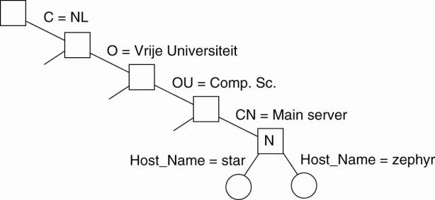
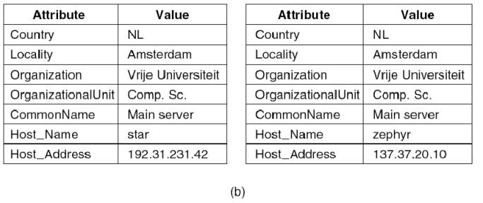
Node N corresponds to the directory entry shown in Fig. 5-22. At the same time, this node acts as a parent to a number of other directory entries that have an additional naming attribute Host_Name that is used as an RDN. For example, such entries may be used to represent hosts as shown in Fig. 5-23(b).

A node in an LDAP naming graph can thus simultaneously represent a directory in the traditional sense as we discussed previously, as well as an LDAP record. This distinction is supported by two different lookup operations. The read operation is used to read a single record given its path name in the DIT. In contrast, the list operation is used to list the names of all outgoing edges of a given node in the DIT. Each name corresponds to a child node of the given node. Note that the list operation does not return any records; it merely returns names. In other words, calling read with as input the name

[Page 221]

/C=NL/O=Vrije Universiteit/OU=Comp. Sc./CN=Main server

will return the record shown in Fig. 5-22, whereas calling list will return the names star and zephyr from the entries shown in Fig. 5-23(b) as well as the names of other hosts that have been registered in a similar way.

Implementing an LDAP directory service proceeds in much the same way as implementing a naming service such as DNS, except that LDAP supports more lookup operations as we will discuss shortly. When dealing with a large-scale directory, the DIT is usually partitioned and distributed across several servers, known as directory service agents (DSA). Each part of a partitioned DIT thus corresponds to a zone in DNS. Likewise, each DSA behaves very much the same as a normal name server, except that it implements a number of typical directory services, such as advanced search operations.

Clients are represented by what are called directory user agents, or simply DUAs. A DUA is similar to a name resolver in structured-naming services. A DUA exchanges information with a DSA according to a standardized access protocol.

What makes an LDAP implementation different from a DNS implementation are the facilities for searching through a DIB. In particular, facilities are provided to search for a directory entry given a set of criteria that attributes of the searched entries should meet. For example, suppose that we want a list of all main servers at the Vrije Universiteit. Using the notation defined in Howes (1997), such a list can be returned using a search operation such as

answer = search("&(C=NL)(O=Vrije Universiteit)(OU=*)(CN=Main server)")

In this example, we have specified that the place to look for main servers is the organization named Vrije Universiteit in country NL, but that we are not interested in a particular organizational unit. However, each returned result should have the CN attribute equal to Main server.

As we already mentioned, searching in a directory service is generally an expensive operation. For example, to find all main servers at the Vrije Universiteit requires searching all entries at each department and combining the results in a single answer. In other words, we will generally need to access several leaf nodes of a DIT in order to get an answer. In practice, this also means that several DSAs need to be accessed. In contrast, naming services can often be implemented in such a way that a lookup operation requires accessing only a single leaf node.

This whole setup of LDAP can be taken one step further by allowing several trees to co-exist, while also being linked to each other. This approach is followed in Microsoft's Active Directory leading to a forest of LDAP domains (Allen and Lowe-Norris, 2003). Obviously, searching in such an organization can be overwhelmingly complex. To circumvent some of the scalability problems, Active Directory usually assumes there is a global index server (called a global catalog) that can be searched first. The index will indicate which LDAP domains need to be searched further.

[Page 222]

Although LDAP by itself already exploits hierarchy for scalability, it is common to combine LDAP with DNS. For example, every tree in LDAP needs to be accessible at the root (known in Active Directory as a domain controller). The root is often known under a DNS name, which, in turn, can be found through an appropriate SRV record as we explained above.

LDAP typically represents a standard way of supporting attribute-based naming. Other recent directory services following this more traditional approach have been developed as well, notably in the context of grid computing and Web services. One specific example is the universal directory and discovery integration or simply UDDI.

These services assume an implementation in which one, or otherwise only a few nodes cooperate to maintain a simple distributed database. From a technological point of view, there is no real novelty here. Likewise, there is also nothing really new to report when it comes to introducing terminology, as can be readily observed when going through the hundreds of pages of the UDDI specifications (Clement et al., 2004). The fundamental scheme is always the same: scalability is achieved by making several of these databases accessible to applications, which are then responsible for querying each database separately and aggregating the results. So much for middleware support.

5.4.3. Decentralized Implementations

With the advent of peer-to-peer systems, researchers have also been looking for solutions for decentralized attribute-based naming systems. The key issue here is that (attribute, value) pairs need to be efficiently mapped so that searching can be done efficiently, that is, by avoiding an exhaustive search through the entire attribute space. In the following we will take a look at several ways how to establish such a mapping.

Mapping to Distributed Hash Tables

Let us first consider the case where (attribute, value) pairs need to be supported by a DHT-based system. First, assume that queries consist of a conjunction of pairs as with LDAP, that is, a user specifies a list of attributes, along with the unique value he wants to see for every respective attribute. The main advantage of this type of query is that no ranges need to be supported. Range queries may significantly increase the complexity of mapping pairs to a DHT.

Single-valued queries are supported in the INS/Twine system (Balazinska et al., 2002). Each entity (referred to as a resource) is assumed to be described by means of possibly hierarchically organized attributes such as shown in Fig. 5-24.

[Page 223]

Figure 5-24. (a) A general description of a resource. (b) Its representation as an AVTree.

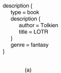
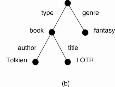
Each such description is translated into an attribute-value tree (AVTree) which is then used as the basis for an encoding that maps well onto a DHT-based system.

The main issue is to transform the AVTrees into a collection of keys that can be looked up in a DHT system. In this case, every path originating in the root is assigned a unique hash value, where a path description starts with a link (representing an attribute), and ends either in a node (value), or another link. Taking Fig. 5-24(b) as our example, the following hashes of all such paths are considered:

h1: hash(type-book)

h2: hash(type-book-author)

h3: hash(type-book-author-Tolkien)

h4: hash(type-book-title)

h5: hash(type-book-title-LOTR)

h6: hash(genre-fantasy)

A node responsible for hash value hi will keep (a reference to) the actual resource. In our example, this may lead to six nodes storing information on Tolkien's Lord of the Rings. However, the benefit of this redundancy is that it will allow supporting partial queries. For example, consider a query such as "Return books written by Tolkien." This query is translated into the AVTree shown in Fig. 5-25 leading to computing the following three hashes:

h1: hash(type-book)

h2: hash(type-book-author)

h3: hash(type-book-author-Tolkien)

Figure 5-25. (a) The resource description of a query. (b) Its representation as an AVTree.

(This item is displayed on page 224 in the print version)

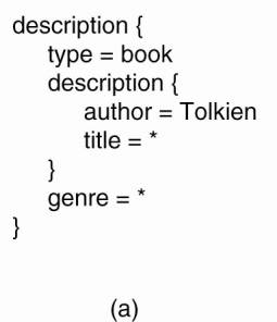
These values will be sent to nodes that store information on Tolkien's books, and will at least return Lord of the Rings. Note that a hash such as h1 is rather general and will be generated often. These type of hashes can be filtered out of the system. Moreover, it is not difficult to see that only the most specific hashes need to be evaluated. Further details can be found in Balzinska et al. (2002).

Now let's take a look at another type of query, namely those that can contain range specifications for attribute values. For example, someone looking for a house will generally want to specify that the price must fall within a specific range. Again, several solutions have been proposed and we will come across some of them when discussing publish/subscribe systems in Chap. 13. Here, we discuss a solution adopted in the SWORD resource discovery system (Oppenheimer et al., 2005).

[Page 224]

In SWORD, (attribute, value) pairs as provided by a resource description are first transformed into a key for a DHT. Note that these pairs always contain a single value; only queries may contain value ranges for attributes. When computing the hash, the name of the attribute and its value are kept separate. In other words, specific bits in the resulting key will identify the attribute name, while others identify its value. In addition, the key will contain a number of random bits to guarantee uniqueness among all keys that need to be generated.

In this way, the space of attributes is conveniently partitioned: if n bits are reserved to code attribute names, 2n different server groups can be used, one group for each attribute name. Likewise, by using m bits to encode values, a further partitioning per server group can be applied to store specific (attribute, value) pairs. DHTs are used only for distributing attribute names.

For each attribute name, the possible range of its value is partitioned into subranges and a single server is assigned to each subrange. To explain, consider a resource description with two attributes: a1 taking values in the range [1..10] and a2 taking values in the range [101...200]. Assume there are two servers for a1 : s11 takes care of recording values of a1 in [1..5], and s12 for values in [6..10]. Likewise, server s21 records values for a2 in range [101..150] and server s22 for values in [151..200]. Then, when the resource gets values (a1 = 7,a2 = 175), server s12 and server s22 will have to be informed.

The advantage of this scheme is that range queries can be easily supported. When a query is issued to return resources that have a2 lying between 165 and 189, the query can be forwarded to server s22 who can then return the resources that match the query range. The drawback, however, is that updates need to be sent to multiple servers. Moreover, it is not immediately clear how well the load is balanced between the various servers. In particular, if certain range queries turn out to be very popular, specific servers will receive a high fraction of all queries. How this load-balancing problem can be tackled for DHT-based systems is discussed in Bharambe at al. (2004).

[Page 225]

Semantic Overlay Networks

The decentralized implementations of attribute-based naming already show an increasing degree of autonomy of the various nodes. The system is less sensitive to nodes joining and leaving in comparison to, for example, distributed LDAP-based systems. This degree of autonomy is further increased when nodes have descriptions of resources that are there to be discovered by others. In other words, there is no a priori deterministic scheme by which (attribute, value) pairs are spread across a collection of nodes.

Not having such a scheme forces nodes to discover where requested resources are. Such a discovery is typical for unstructured overlay networks, which we already discussed in Chap. 2. In order to make searching efficient, it is important that a node has references to others that can most likely answer its queries. If we make the assumption that queries originating from node P are strongly related to the resources that P has, then we are seeking to provide P with a collection of links to semantically proximal neighbors. Recall that such a list is also known as a partial view. Semantical proximity can be defined in different ways, but it boils down to keeping track of nodes with similar resources. The nodes and these links will then form what is known as a semantic overlay network.

A common approach to semantic overlay networks is to assume that there is commonality in the meta information maintained at each node. In other words, the resources stored at each node are described using the same collection of attributes, or, more precisely, the same data schema (Crespo and Garcia-Molina, 2003). Having such a schema will allow defining specific similarity functions between nodes. Each node will then keep only links to the K most similar neighbors and query those nodes first when looking for specific data. Note that this approach makes sense only if we can generally assume that a query initiated at a node relates to the content stored at that node.

Unfortunately, assuming commonality in data schemas is generally wrong. In practice, the meta information on resources is highly inconsistent across different nodes and reaching consensus and what and how to describe resources is close to impossible. For this reason, semantic overlay networks will generally need to find different ways to define similarity.

One approach is to forget about attributes altogether and consider only very simple descriptors such as file names. Passively constructing an overlay can be done by keeping track of which nodes respond positively to file searches. For example, Sripanidkulchai et al. (2003) first send a query to a node's semantic neigh-bors, but if the requested file is not there a (limited) broadcast is then done. Of course, such a broadcast may lead to an update of the semantic-neighbors list. As a note, it is interesting to see that if a node requests its semantic neighbors to forward a query to their semantic neighbors, that the effect is minimal (Handrukande et al., 2004). This phenomenon can be explained by what is known as the smallworld effect which essentially states that the friends of Alice are also each other's friends (Watts, 1999).

[Page 226]

A more proactive approach toward constructing a semantic-neighbor list is proposed by Voulgaris and van Steen (2005) who use a simple semantic proximity function defined on the file lists FLP and FLQ of two nodes P and Q, respectively. This function simply counts the number of common files in FLP and FLQ. The goal is then to optimize the proximity function by letting a node keep a list of only those neighbors that have the most files in common with it.

To this end, a two-layered gossiping scheme is deployed as shown in Fig. 5-26. The bottom layer consists of an epidemic protocol that aims at maintaining a partial view of uniform randomly-selected nodes. There are different ways to achieve this as we explained in Chap. 2 [see also Jelasity et al. (2005a)]. The top layer maintains a list of semantically proximal neighbors through gossiping. To initiate an exchange, an node P can randomly select a neighbor Q from its current list, but the trick is to let P send only those entries that are semantically closest to Q. In turn, when P receives entries from Q, it will eventually keep a partial view consisting only of the semantically closest nodes. As it turns out, the partial views as maintained by the top layer will rapidly converge to an optimum.

Figure 5-26. Maintaining a semantic overlay through gossiping.

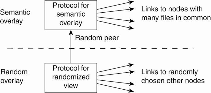
As will have become clear by now, semantic overlay networks are closely related to decentralized searching. An extensive overview of searching in all kinds of peer-to-peer systems is discussed in Risson and Moors (2006).