Chapter 6. Synchronization

In the previous chapters, we have looked at processes and communication between processes. While communication is important, it is not the entire story. Closely related is how processes cooperate and synchronize with one another. Cooperation is partly supported by means of naming, which allows processes to at least share resources, or entities in general.

In this chapter, we mainly concentrate on how processes can synchronize. For example, it is important that multiple processes do not simultaneously access a shared resource, such as printer, but instead cooperate in granting each other temporary exclusive access. Another example is that multiple processes may sometimes need to agree on the ordering of events, such as whether message m1 from process P was sent before or after message m2 from process Q.

As it turns out, synchronization in distributed systems is often much more difficult compared to synchronization in uniprocessor or multiprocessor systems. The problems and solutions that are discussed in this chapter are, by their nature, rather general, and occur in many different situations in distributed systems.

We start with a discussion of the issue of synchronization based on actual time, followed by synchronization in which only relative ordering matters rather than ordering in absolute time.

In many cases, it is important that a group of processes can appoint one process as a coordinator, which can be done by means of election algorithms. We discuss various election algorithms in a separate section.

[Page 232]

Distributed algorithms come in all sorts and flavors and have been developed for very different types of distributed systems. Many examples (and further references) can be found in Andrews (2000) and Guerraoui and Rodrigues (2006). More formal approaches to a wealth of algorithms can be found in text books from Attiya and Welch (2004), Lynch (1996), and (Tel, 2000).

6.1. Clock Synchronization

In a centralized system, time is unambiguous. When a process wants to know the time, it makes a system call and the kernel tells it. If process A asks for the time, and then a little later process B asks for the time, the value that B gets will be higher than (or possibly equal to) the value A got. It will certainly not be lower. In a distributed system, achieving agreement on time is not trivial.

Just think, for a moment, about the implications of the lack of global time on the UNIX make program, as a single example. Normally, in UNIX, large programs are split up into multiple source files, so that a change to one source file only requires one file to be recompiled, not all the files. If a program consists of 100 files, not having to recompile everything because one file has been changed greatly increases the speed at which programmers can work.

The way make normally works is simple. When the programmer has finished changing all the source files, he runs make, which examines the times at which all the source and object files were last modified. If the source file input.c has time 2151 and the corresponding object file input.o has time 2150, make knows that input.c has been changed since input.o was created, and thus input.c must be recompiled. On the other hand, if output.c has time 2144 and output.o has time 2145, no compilation is needed. Thus make goes through all the source files to find out which ones need to be recompiled and calls the compiler to recompile them.

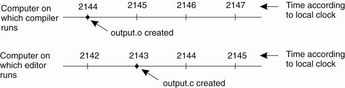
Now imagine what could happen in a distributed system in which there were no global agreement on time. Suppose that output.o has time 2144 as above, and shortly thereafter output.c is modified but is assigned time 2143 because the clock on its machine is slightly behind, as shown in Fig. 6-1. Make will not call the compiler. The resulting executable binary program will then contain a mixture of object files from the old sources and the new sources. It will probably crash and the programmer will go crazy trying to understand what is wrong with the code.

Figure 6-1. When each machine has its own clock, an event that occurred after another event may nevertheless be assigned an earlier time.

(This item is displayed on page 233 in the print version)

There are many more examples where an accurate account of time is needed. The example above can easily be reformulated to file timestamps in general. In addition, think of application domains such as financial brokerage, security auditing, and collaborative sensing, and it will become clear that accurate timing is important. Since time is so basic to the way people think and the effect of not having all the clocks synchronized can be so dramatic, it is fitting that we begin our study of synchronization with the simple question: Is it possible to synchronize all the clocks in a distributed system? The answer is surprisingly complicated.

[Page 233]

6.1.1. Physical Clocks

Nearly all computers have a circuit for keeping track of time. Despite the widespread use of the word "clock" to refer to these devices, they are not actually clocks in the usual sense. Timer is perhaps a better word. A computer timer is usually a precisely machined quartz crystal. When kept under tension, quartz crystals oscillate at a well-defined frequency that depends on the kind of crystal, how it is cut, and the amount of tension. Associated with each crystal are two registers, a counter and a holding register. Each oscillation of the crystal decrements the counter by one. When the counter gets to zero, an interrupt is generated and the counter is reloaded from the holding register. In this way, it is possible to program a timer to generate an interrupt 60 times a second, or at any other desired frequency. Each interrupt is called one clock tick.

When the system is booted, it usually asks the user to enter the date and time, which is then converted to the number of ticks after some known starting date and stored in memory. Most computers have a special battery-backed up CMOS RAM so that the date and time need not be entered on subsequent boots. At every clock tick, the interrupt service procedure adds one to the time stored in memory. In this way, the (software) clock is kept up to date.

With a single computer and a single clock, it does not matter much if this clock is off by a small amount. Since all processes on the machine use the same clock, they will still be internally consistent. For example, if the file input.c has time 2151 and file input.o has time 2150, make will recompile the source file, even if the clock is off by 2 and the true times are 2153 and 2152, respectively. All that really matters are the relative times.

As soon as multiple CPUs are introduced, each with its own clock, the situation changes radically. Although the frequency at which a crystal oscillator runs is usually fairly stable, it is impossible to guarantee that the crystals in different computers all run at exactly the same frequency. In practice, when a system has n computers, all n crystals will run at slightly different rates, causing the (software) clocks gradually to get out of synch and give different values when read out. This difference in time values is called clock skew. As a consequence of this clock skew, programs that expect the time associated with a file, object, process, or message to be correct and independent of the machine on which it was generated (i.e., which clock it used) can fail, as we saw in the make example above.

[Page 234]

In some systems (e.g., real-time systems), the actual clock time is important. Under these circumstances, external physical clocks are needed. For reasons of efficiency and redundancy, multiple physical clocks are generally considered desirable, which yields two problems: (1) How do we synchronize them with real-world clocks, and (2) How do we synchronize the clocks with each other?

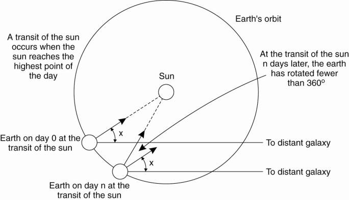
Before answering these questions, let us digress slightly to see how time is actually measured. It is not nearly as easy as one might think, especially when high accuracy is required. Since the invention of mechanical clocks in the 17th century, time has been measured astronomically. Every day, the sun appears to rise on the eastern horizon, then climbs to a maximum height in the sky, and finally sinks in the west. The event of the sun's reaching its highest apparent point in the sky is called the transit of the sun. This event occurs at about noon each day. The interval between two consecutive transits of the sun is called the solar day. Since there are 24 hours in a day, each containing 3600 seconds, the solar second is defined as exactly 1/86400th of a solar day. The geometry of the mean solar day calculation is shown in Fig. 6-2.

Figure 6-2. Computation of the mean solar day.

In the 1940s, it was established that the period of the earth's rotation is not constant. The earth is slowing down due to tidal friction and atmospheric drag. Based on studies of growth patterns in ancient coral, geologists now believe that 300 million years ago there were about 400 days per year. The length of the year (the time for one trip around the sun) is not thought to have changed; the day has simply become longer. In addition to this long-term trend, short-term variations in the length of the day also occur, probably caused by turbulence deep in the earth's core of molten iron. These revelations led astronomers to compute the length of the day by measuring a large number of days and taking the average before dividing by 86,400. The resulting quantity was called the mean solar second.

[Page 235]

With the invention of the atomic clock in 1948, it became possible to measure time much more accurately, and independent of the wiggling and wobbling of the earth, by counting transitions of the cesium 133 atom. The physicists took over the job of timekeeping from the astronomers and defined the second to be the time it takes the cesium 133 atom to make exactly 9,192,631,770 transitions. The choice of 9,192,631,770 was made to make the atomic second equal to the mean solar second in the year of its introduction. Currently, several laboratories around the world have cesium 133 clocks. Periodically, each laboratory tells the Bureau International de l'Heure (BIH) in Paris how many times its clock has ticked. The BIH averages these to produce International Atomic Time, which is abbreviated TAI. Thus TAI is just the mean number of ticks of the cesium 133 clocks since midnight on Jan. 1, 1958 (the beginning of time) divided by 9,192,631,770.

Although TAI is highly stable and available to anyone who wants to go to the trouble of buying a cesium clock, there is a serious problem with it; 86,400 TAI seconds is now about 3 msec less than a mean solar day (because the mean solar day is getting longer all the time). Using TAI for keeping time would mean that over the course of the years, noon would get earlier and earlier, until it would eventually occur in the wee hours of the morning. People might notice this and we could have the same kind of situation as occurred in 1582 when Pope Gregory XIII decreed that 10 days be omitted from the calendar. This event caused riots in the streets because landlords demanded a full month's rent and bankers a full month's interest, while employers refused to pay workers for the 10 days they did not work, to mention only a few of the conflicts. The Protestant countries, as a matter of principle, refused to have anything to do with papal decrees and did not accept the Gregorian calendar for 170 years.

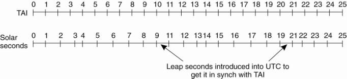
BIH solves the problem by introducing leap seconds whenever the discrepancy between TAI and solar time grows to 800 msec. The use of leap seconds is illustrated in Fig. 6-3. This correction gives rise to a time system based on constant TAI seconds but which stays in phase with the apparent motion of the sun. It is called Universal Coordinated Time, but is abbreviated as UTC. UTC is the basis of all modern civil timekeeping. It has essentially replaced the old standard, Greenwich Mean Time, which is astronomical time.

[Page 236]

Figure 6-3. TAI seconds are of constant length, unlike solar seconds. Leap seconds are introduced when necessary to keep in phase with the sun.

(This item is displayed on page 235 in the print version)

Most electric power companies synchronize the timing of their 60-Hz or 50-Hz clocks to UTC, so when BIH announces a leap second, the power companies raise their frequency to 61 Hz or 51 Hz for 60 or 50 sec, to advance all the clocks in their distribution area. Since 1 sec is a noticeable interval for a computer, an operating system that needs to keep accurate time over a period of years must have special software to account for leap seconds as they are announced (unless they use the power line for time, which is usually too crude). The total number of leap seconds introduced into UTC so far is about 30.

To provide UTC to people who need precise time, the National Institute of Standard Time (NIST) operates a shortwave radio station with call letters WWV from Fort Collins, Colorado. WWV broadcasts a short pulse at the start of each UTC second. The accuracy of WWV itself is about ±1 msec, but due to random atmospheric fluctuations that can affect the length of the signal path, in practice the accuracy is no better than ±10 msec. In England, the station MSF, operating from Rugby, Warwickshire, provides a similar service, as do stations in several other countries.

Several earth satellites also offer a UTC service. The Geostationary Environment Operational Satellite can provide UTC accurately to 0.5 msec, and some other satellites do even better.

Using either shortwave radio or satellite services requires an accurate know-ledge of the relative position of the sender and receiver, in order to compensate for the signal propagation delay. Radio receivers for WWV, GEOS, and the other UTC sources are commercially available.

6.1.2. Global Positioning System

As a step toward actual clock synchronization problems, we first consider a related problem, namely determining one's geographical position anywhere on Earth. This positioning problem is by itself solved through a highly specific, dedicated distributed system, namely GPS, which is an acronym for global positioning system. GPS is a satellite-based distributed system that was launched in 1978. Although it has been used mainly for military applications, in recent years it has found its way to many civilian applications, notably for traffic navigation. However, many more application domains exist. For example, GPS phones now allow to let callers track each other's position, a feature which may show to be extremely handy when you are lost or in trouble. This principle can easily be applied to tracking other things as well, including pets, children, cars, boats, and so on. An excellent overview of GPS is provided by Zogg (2002).

[Page 237]

GPS uses 29 satellites each circulating in an orbit at a height of approximately 20,000 km. Each satellite has up to four atomic clocks, which are regularly calibrated from special stations on Earth. A satellite continuously broadcasts its position, and time stamps each message with its local time. This broadcasting allows every receiver on Earth to accurately compute its own position using, in principle, only three satellites. To explain, let us first assume that all clocks, including the receiver's, are synchronized.

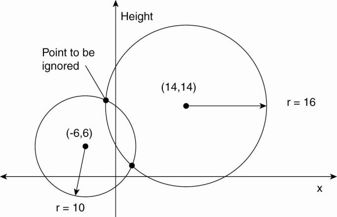
In order to compute a position, consider first the two-dimensional case, as shown in Fig. 6-4, in which two satellites are drawn, along with the circles representing points at the same distance from each respective satellite. The y-axis represents the height, while the x-axis represents a straight line along the Earth's surface at sea level. Ignoring the highest point, we see that the intersection of the two circles is a unique point (in this case, perhaps somewhere up a mountain).

Figure 6-4. Computing a position in a two-dimensional space.

This principle of intersecting circles can be expanded to three dimensions, meaning that we need three satellites to determine the longitude, latitude, and altitude of a receiver on Earth. This positioning is all fairly straightforward, but matters become complicated when we can no longer assume that all clocks are perfectly synchronized.

There are two important real-world facts that we need to take into account:

It takes a while before data on a satellite's position reaches the receiver.

The receiver's clock is generally not in synch with that of a satellite.

Assume that the timestamp from a satellite is completely accurate. Let Δr denote the deviation of the receiver's clock from the actual time. When a message is received from satellite i with timestamp Ti, then the measured delay Δi by the receiver consists of two components: the actual delay, along with its own deviation:

[Page 238]

Δi = (Tnow - Ti) + Δr

As signals travel with the speed of light, c, the measured distance of the satellite is clearly cΔi. With

di = c(Tnow - Ti)

being the real distance between the receiver and the satellite, the measured distance can be rewritten to di + cΔr. The real distance is simply computed as:

where xi, yi, and zi denote the coordinates of satellite i. What we see now is that if we have four satellites, we get four equations in four unknowns, allowing us to solve the coordinates xr, yr, and zr for the receiver, but also Δr. In other words, a GPS measurement will also give an account of the actual time. Later in this chapter we will return to determining positions following a similar approach.

So far, we have assumed that measurements are perfectly accurate. Of course, they are not. For one thing, GPS does not take leap seconds into account. In other words, there is a systematic deviation from UTC, which by January 1, 2006 is 14 seconds. Such an error can be easily compensated for in software. However, there are many other sources of errors, starting with the fact that the atomic clocks in the satellites are not always in perfect synch, the position of a satellite is not known precisely, the receiver's clock has a finite accuracy, the signal propagation speed is not constant (as signals slow down when entering, e.g., the ionosphere), and so on. Moreover, we all know that the earth is not a perfect sphere, leading to further corrections.

By and large, computing an accurate position is far from a trivial undertaking and requires going down into many gory details. Nevertheless, even with relatively cheap GPS receivers, positioning can be precise within a range of 1–5 meters. Moreover, professional receivers (which can easily be hooked up in a computer network) have a claimed error of less than 20–35 nanoseconds. Again, we refer to the excellent overview by Zogg (2002) as a first step toward getting acquainted with the details.

6.1.3. Clock Synchronization Algorithms

If one machine has a WWV receiver, the goal becomes keeping all the other machines synchronized to it. If no machines have WWV receivers, each machine keeps track of its own time, and the goal is to keep all the machines together as well as possible. Many algorithms have been proposed for doing this synchronization. A survey is given in Ramanathan et al. (1990).

[Page 239]

All the algorithms have the same underlying model of the system. Each machine is assumed to have a timer that causes an interrupt H times a second. When this timer goes off, the interrupt handler adds 1 to a software clock that keeps track of the number of ticks (interrupts) since some agreed-upon time in the past. Let us call the value of this clock C. More specifically, when the UTC time is t, the value of the clock on machine p is Cp(t). In a perfect world, we would have Cp(t) = t for all p and all t. In other words, ideally should be 1. is called the frequency of p's clock at time t. The skew of the clock is defined as and denotes the extent to which the frequency differs from that of a perfect clock. The offset relative to a specific time t is Cp(t) - t.

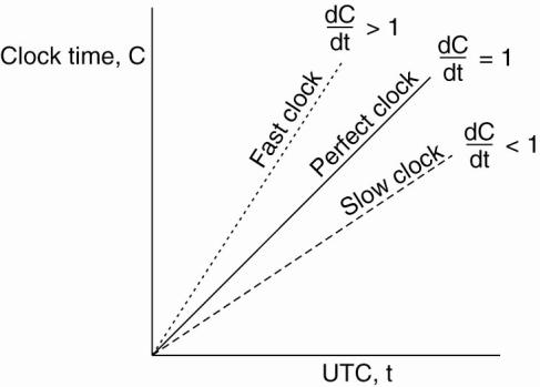
Real timers do not interrupt exactly H times a second. Theoretically, a timer with H = 60 should generate 216,000 ticks per hour. In practice, the relative error obtainable with modern timer chips is about 10-5, meaning that a particular machine can get a value in the range 215,998 to 216,002 ticks per hour. More precisely, if there exists some constant ρ such that

the timer can be said to be working within its specification. The constant ρ is specified by the manufacturer and is known as the maximum drift rate. Note that the maximum drift rate specifies to what extent a clock's skew is allowed to fluctuate. Slow, perfect, and fast clocks are shown in Fig. 6-5.

Figure 6-5. The relation between clock time and UTC when clocks tick at different rates.

If two clocks are drifting from UTC in the opposite direction, at a time Δt after they were synchronized, they may be as much as 2ρ Δt apart. If the operating system designers want to guarantee that no two clocks ever differ by more than δ, clocks must be resynchronized (in software) at least every δ/2ρ seconds. The various algorithms differ in precisely how this resynchronization is done.

[Page 240]

Network Time Protocol

A common approach in many protocols and originally proposed by Cristian (1989) is to let clients contact a time server. The latter can accurately provide the current time, for example, because it is equipped with a WWV receiver or an accurate clock. The problem, of course, is that when contacting the server, message delays will have outdated the reported time. The trick is to find a good estimation for these delays. Consider the situation sketched in Fig. 6-6.

Figure 6-6. Getting the current time from a time server.

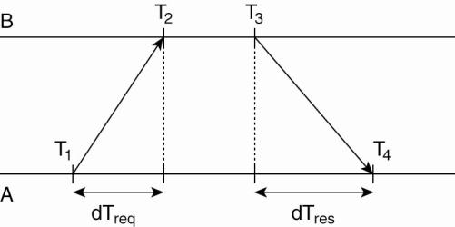
In this case, A will send a request to B, timestamped with value T1 . B, in turn, will record the time of receipt T2 (taken from its own local clock), and returns a response timestamped with value T3, and piggybacking the previously recorded value T2. Finally, A records the time of the response's arrival, T4. Let us assume that the propagation delays from A to B is roughly the same as B to A, meaning that T2 - T1 T4 -T3. In that case, A can estimate its offset relative to B as

Of course, time is not allowed to run backward. If A's clock is fast, θ < 0, meaning that A should, in principle, set its clock backward. This is not allowed as it could cause serious problems such as an object file compiled just after the clock change having a time earlier than the source which was modified just before the clock change.

Such a change must be introduced gradually. One way is as follows. Suppose that the timer is set to generate 100 interrupts per second. Normally, each interrupt would add 10 msec to the time. When slowing down, the interrupt routine adds only 9 msec each time until the correction has been made. Similarly, the clock can be advanced gradually by adding 11 msec at each interrupt instead of jumping it forward all at once.

In the case of the network time protocol (NTP), this protocol is set up pair-wise between servers. In other words, B will also probe A for its current time. The offset θ is computed as given above, along with the estimation δ for the delay:

[Page 241]

Eight pairs of (θ,δ) values are buffered, finally taking the minimal value found for δ as the best estimation for the delay between the two servers, and subsequently the associated value θ as the most reliable estimation of the offset.

Applying NTP symmetrically should, in principle, also let B adjust its clock to that of A. However, if B's clock is known to be more accurate, then such an adjustment would be foolish. To solve this problem, NTP divides servers into strata. A server with a reference clock such as a WWV receiver or an atomic clock, is known to be a stratum-1 server (the clock itself is said to operate at stratum 0). When A contacts B, it will only adjust its time if its own stratum level is higher than that of B. Moreover, after the synchronization, A's stratum level will become one higher than that of B. In other words, if B is a stratum-k server, then A will become a stratum-(k+1) server if its original stratum level was already larger than k. Due to the symmetry of NTP, if A's stratum level was lower than that of B, B will adjust itself to A.

There are many important features about NTP, of which many relate to identifying and masking errors, but also security attacks. NTP is described in Mills (1992) and is known to achieve (worldwide) accuracy in the range of 1–50 msec. The newest version (NTPv4) was initially documented only by means of its implementation, but a detailed description can now be found in Mills (2006).

The Berkeley Algorithm

In many algorithms such as NTP, the time server is passive. Other machines periodically ask it for the time. All it does is respond to their queries. In Berkeley UNIX, exactly the opposite approach is taken (Gusella and Zatti, 1989). Here the time server (actually, a time daemon) is active, polling every machine from time to time to ask what time it is there. Based on the answers, it computes an average time and tells all the other machines to advance their clocks to the new time or slow their clocks down until some specified reduction has been achieved. This method is suitable for a system in which no machine has a WWV receiver. The time daemon's time must be set manually by the operator periodically. The method is illustrated in Fig. 6-7.

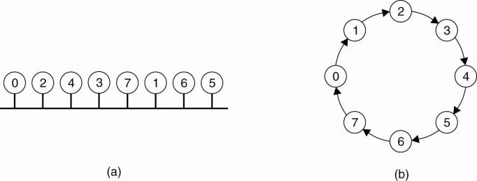
Figure 6-7. (a) The time daemon asks all the other machines for their clock values. (b) The machines answer. (c) The time daemon tells everyone how to adjust their clock.

(This item is displayed on page 242 in the print version)

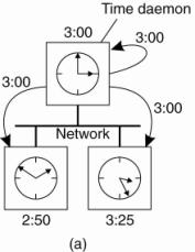
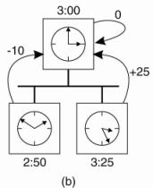
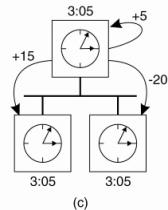
In Fig. 6-7(a), at 3:00, the time daemon tells the other machines its time and asks for theirs. In Fig. 6-7(b), they respond with how far ahead or behind the time daemon they are. Armed with these numbers, the time daemon computes the average and tells each machine how to adjust its clock [see Fig. 6-7(c)].

Note that for many purposes, it is sufficient that all machines agree on the same time. It is not essential that this time also agrees with the real time as announced on the radio every hour. If in our example of Fig. 6-7 the time daemon's clock would never be manually calibrated, no harm is done provided none of the other nodes communicates with external computers. Everyone will just happily agree on a current time, without that value having any relation with reality.

[Page 242]

Clock Synchronization in Wireless Networks

An important advantage of more traditional distributed systems is that we can easily and efficiently deploy time servers. Moreover, most machines can contact each other, allowing for a relatively simple dissemination of information. These assumptions are no longer valid in many wireless networks, notably sensor networks. Nodes are resource constrained, and multihop routing is expensive. In addition, it is often important to optimize algorithms for energy consumption. These and other observations have led to the design of very different clock synchronization algorithms for wireless networks. In the following, we consider one specific solution. Sivrikaya and Yener (2004) provide a brief overview of other solutions. An extensive survey can be found in Sundararaman et al. (2005).

Reference broadcast synchronization (RBS) is a clock synchronization protocol that is quite different from other proposals (Elson et al., 2002). First, the protocol does not assume that there is a single node with an accurate account of the actual time available. Instead of aiming to provide all nodes UTC time, it aims at merely internally synchronizing the clocks, just as the Berkeley algorithm does. Second, the solutions we have discussed so far are designed to bring the sender and receiver into synch, essentially following a two-way protocol. RBS deviates from this pattern by letting only the receivers synchronize, keeping the sender out of the loop.

In RBS, a sender broadcasts a reference message that will allow its receivers to adjust their clocks. A key observation is that in a sensor network the time to propagate a signal to other nodes is roughly constant, provided no multi-hop routing is assumed. Propagation time in this case is measured from the moment that a message leaves the network interface of the sender. As a consequence, two important sources for variation in message transfer no longer play a role in estimating delays: the time spent to construct a message, and the time spent to access the network. This principle is shown in Fig. 6-8.

[Page 243]

Figure 6-8. (a) The usual critical path in determining network delays. (b) The critical path in the case of RBS.

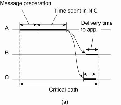
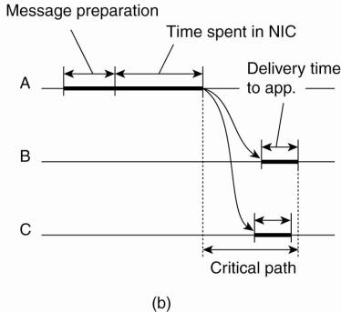
Note that in protocols such as NTP, a timestamp is added to the message before it is passed on the network interface. Furthermore, as wireless networks are based on a contention protocol, there is generally no saying how long it will take before a message can actually be transmitted. These factors of nondeterminism are eliminated in RBS. What remains is the delivery time at the receiver, but this time varies considerably less than the network-access time.

The idea underlying RBS is simple: when a node broadcasts a reference message m, each node p simply records the time Tp,m that it received m. Note that Tp,m is read from p's local clock. Ignoring clock skew, two nodes p and q can exchange each other's delivery times in order to estimate their mutual, relative offset:

where M is the total number of reference messages sent. This information is important: node p will know the value of q's clock relative to its own value. Moreover, if it simply stores these offsets, there is no need to adjust its own clock, which saves energy.

Unfortunately, clocks can drift apart. The effect is that simply computing the average offset as done above will not work: the last values sent are simply less accurate than the first ones. Moreover, as time goes by, the offset will presumably increase. Elson et al. use a very simple algorithm to compensate for this: instead of computing an average they apply standard linear regression to compute the offset as a function:

[Page 244]

Offset [p,q](t) = αt+β

The constants α and β are computed from the pairs (Tp,k,Tq,k). This new form will allow a much more accurate computation of q's current clock value by node p, and vice versa.

6.2. Logical Clocks

So far, we have assumed that clock synchronization is naturally related to real time. However, we have also seen that it may be sufficient that every node agrees on a current time, without that time necessarily being the same as the real time. We can go one step further. For running make, for example, it is adequate that two nodes agree that input.o is outdated by a new version of input.c. In this case, keeping track of each other's events (such as a producing a new version of input.c) is what matters. For these algorithms, it is conventional to speak of the clocks as logical clocks.

In a classic paper, Lamport (1978) showed that although clock synchronization is possible, it need not be absolute. If two processes do not interact, it is not necessary that their clocks be synchronized because the lack of synchronization would not be observable and thus could not cause problems. Furthermore, he pointed out that what usually matters is not that all processes agree on exactly what time it is, but rather that they agree on the order in which events occur. In the make example, what counts is whether input.c is older or newer than input.o, not their absolute creation times.

In this section we will discuss Lamport's algorithm, which synchronizes logical clocks. Also, we discuss an extension to Lamport's approach, called vector timestamps.

6.2.1. Lamport's Logical Clocks

To synchronize logical clocks, Lamport defined a relation called happens-before. The expression a b is read "a happens before b" and means that all processes agree that first event a occurs, then afterward, event b occurs. The happens-before relation can be observed directly in two situations:

If a and b are events in the same process, and a occurs before b, then a b is true.

If a is the event of a message being sent by one process, and b is the event of the message being received by another process, then a b is also true. A message cannot be received before it is sent, or even at the same time it is sent, since it takes a finite, nonzero amount of time to arrive.

[Page 245]

Happens-before is a transitive relation, so if a b and b c, then a c. If two events, x and y, happen in different processes that do not exchange messages (not even indirectly via third parties), then x y is not true, but neither is y x. These events are said to be concurrent, which simply means that nothing can be said (or need be said) about when the events happened or which event happened first.

What we need is a way of measuring a notion of time such that for every event, a, we can assign it a time value C (a) on which all processes agree. These time values must have the property that if a b, then C (a) < C (b). To rephrase the conditions we stated earlier, if a and b are two events within the same process and a occurs before b, then C (a) < C (b). Similarly, if a is the sending of a message by one process and b is the reception of that message by another process, then C (a) and C (b) must be assigned in such a way that everyone agrees on the values of C (a) and C (b) with C (a) < C (b). In addition, the clock time, C, must always go forward (increasing), never backward (decreasing). Corrections to time can be made by adding a positive value, never by subtracting one.

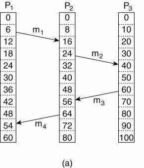
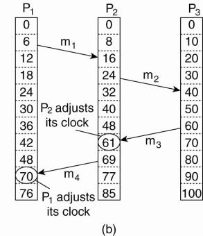
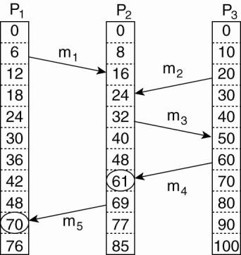
Now let us look at the algorithm Lamport proposed for assigning times to events. Consider the three processes depicted in Fig. 6-9(a). The processes run on different machines, each with its own clock, running at its own speed. As can be seen from the figure, when the clock has ticked 6 times in process P1, it has ticked 8 times in process P2 and 10 times in process P3. Each clock runs at a constant rate, but the rates are different due to differences in the crystals.

Figure 6-9. (a) Three processes, each with its own clock. The clocks run at different rates. (b) Lamport's algorithm corrects the clocks.

[Page 246]

At time 6, process P1 sends message m1 to process P2. How long this message takes to arrive depends on whose clock you believe. In any event, the clock in process P2 reads 16 when it arrives. If the message carries the starting time, 6, in it, process P2 will conclude that it took 10 ticks to make the journey. This value is certainly possible. According to this reasoning, message m2 from P2 to R takes 16 ticks, again a plausible value.

Now consider message m3. It leaves process P3 at 60 and arrives at P2 at 56. Similarly, message m4 from P2 to P1 leaves at 64 and arrives at 54. These values are clearly impossible. It is this situation that must be prevented.

Lamport's solution follows directly from the happens-before relation. Since m3 left at 60, it must arrive at 61 or later. Therefore, each message carries the sending time according to the sender's clock. When a message arrives and the receiver's clock shows a value prior to the time the message was sent, the receiver fast forwards its clock to be one more than the sending time. In Fig. 6-9(b) we see that m3 now arrives at 61. Similarly, m4 arrives at 70.

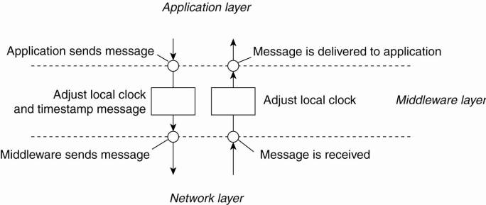
To prepare for our discussion on vector clocks, let us formulate this procedure more precisely. At this point, it is important to distinguish three different layers of software as we already encountered in Chap. 1: the network, a middleware layer, and an application layer, as shown in Fig. 6-10. What follows is typically part of the middleware layer.

Figure 6-10. The positioning of Lamport's logical clocks in distributed systems.

To implement Lamport's logical clocks, each process Pi maintains a local counter Ci. These counters are updated as follows steps (Raynal and Singhal, 1996):

1. Before executing an event (i.e., sending a message over the network, delivering a message to an application, or some other internal event), Pi executes Ci Ci + 1.

2. When process Pi sends a message m to Pj, it sets m's timestamp ts (m) equal to Ci after having executed the previous step.

[Page 247]

3. Upon the receipt of a message m, process Pj adjusts its own local counter as Cj max{Cj, ts (m)}, after which it then executes the first step and delivers the message to the application.

In some situations, an additional requirement is desirable: no two events ever occur at exactly the same time. To achieve this goal, we can attach the number of the process in which the event occurs to the low-order end of the time, separated by a decimal point. For example, an event at time 40 at process Pi will be timestamped with 40.i.

Note that by assigning the event time C (a) Ci(a) if a happened at process Pi at time Ci(a), we have a distributed implementation of the global time value we were initially seeking for.

Example: Totally Ordered Multicasting

As an application of Lamport's logical clocks, consider the situation in which a database has been replicated across several sites. For example, to improve query performance, a bank may place copies of an account database in two different cities, say New York and San Francisco. A query is always forwarded to the nearest copy. The price for a fast response to a query is partly paid in higher update costs, because each update operation must be carried out at each replica.

In fact, there is a more stringent requirement with respect to updates. Assume a customer in San Francisco wants to add $100 to his account, which currently contains $1,000. At the same time, a bank employee in New York initiates an update by which the customer's account is to be increased with 1 percent interest. Both updates should be carried out at both copies of the database. However, due to communication delays in the underlying network, the updates may arrive in the order as shown in Fig. 6-11.

Figure 6-11. Updating a replicated database and leaving it in an inconsistent state.

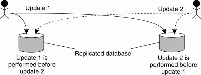
The customer's update operation is performed in San Francisco before the interest update. In contrast, the copy of the account in the New York replica is first updated with the 1 percent interest, and after that with the $100 deposit. Consequently, the San Francisco database will record a total amount of $1,111, whereas the New York database records $1,110.

[Page 248]

The problem that we are faced with is that the two update operations should have been performed in the same order at each copy. Although it makes a difference whether the deposit is processed before the interest update or the other way around, which order is followed is not important from a consistency point of view. The important issue is that both copies should be exactly the same. In general, situations such as these require a totally-ordered multicast, that is, a multicast operation by which all messages are delivered in the same order to each receiver. Lamport's logical clocks can be used to implement totally-ordered multicasts in a completely distributed fashion.

Consider a group of processes multicasting messages to each other. Each message is always timestamped with the current (logical) time of its sender. When a message is multicast, it is conceptually also sent to the sender. In addition, we assume that messages from the same sender are received in the order they were sent, and that no messages are lost.

When a process receives a message, it is put into a local queue, ordered according to its timestamp. The receiver multicasts an acknowledgment to the other processes. Note that if we follow Lamport's algorithm for adjusting local clocks, the timestamp of the received message is lower than the timestamp of the acknowledgment. The interesting aspect of this approach is that all processes will eventually have the same copy of the local queue (provided no messages are removed).

A process can deliver a queued message to the application it is running only when that message is at the head of the queue and has been acknowledged by each other process. At that point, the message is removed from the queue and handed over to the application; the associated acknowledgments can simply be removed. Because each process has the same copy of the queue, all messages are delivered in the same order everywhere. In other words, we have established totally-ordered multicasting.

As we shall see in later chapters, totally-ordered multicasting is an important vehicle for replicated services where the replicas are kept consistent by letting them execute the same operations in the same order everywhere. As the replicas essentially follow the same transitions in the same finite state machine, it is also known as state machine replication (Schneider, 1990).

6.2.2. Vector Clocks

Lamport's logical clocks lead to a situation where all events in a distributed system are totally ordered with the property that if event a happened before event b, then a will also be positioned in that ordering before b, that is, C (a) < C (b).

[Page 249]

However, with Lamport clocks, nothing can be said about the relationship between two events a and b by merely comparing their time values C (a) and C (b), respectively. In other words, if C (a) < C (b), then this does not necessarily imply that a indeed happened before b. Something more is needed for that.

To explain, consider the messages as sent by the three processes shown in Fig. 6-12. Denote by Tsnd (mi) the logical time at which message mi was sent, and likewise, by Trcv (mi) the time of its receipt. By construction, we know that for each message Tsnd (mi) < Trcv (mi). But what can we conclude in general from Trcv (mi) < Tsnd (mj)?

Figure 6-12. Concurrent message transmission using logical clocks.

In the case for which mi=m1 and mj=m3, we know that these values correspond to events that took place at process P2, meaning that m3 was indeed sent after the receipt of message m1. This may indicate that the sending of message m3 depended on what was received through message m1 . However, we also know that Trcv (m1) < Tsnd (m2). However, the sending of m2 has nothing to do with the receipt of m1.

The problem is that Lamport clocks do not capture causality. Causality can be captured by means of vector clocks. A vector clock VC (a) assigned to an event a has the property that if VC (a) < VC (b) for some event b, then event a is known to causally precede event b. Vector clocks are constructed by letting each process Pi maintain a vector VCi with the following two properties:

1. VCi [i ] is the number of events that have occurred so far at Pi. In other words, VCi [i ] is the local logical clock at process Pi.

2. If VCi [j ] = k then Pi knows that k events have occurred at Pj. It is thus Pi's knowledge of the local time at Pj.

The first property is maintained by incrementing VCi [i ] at the occurrence of each new event that happens at process Pi. The second property is maintained by piggybacking vectors along with messages that are sent. In particular, the following steps are performed:

[Page 250]

1. Before executing an event (i.e., sending a message over the network, delivering a message to an application, or some other internal event), Pi executes VCi [i ] VCi [i ] + 1.

2. When process Pi sends a message m to Pj, it sets m's (vector) timestamp ts (m) equal to VCi after having executed the previous step.

3. Upon the receipt of a message m, process Pj adjusts its own vector by setting VCj [k ] max{VCj [k ], ts (m)[k ]} for each k, after which it executes the first step and delivers the message to the application.

Note that if an event a has timestamp ts (a), then ts (a)[i ]-1 denotes the number of events processed at Pi that causally precede a. As a consequence, when Pj receives a message from Pi with timestamp ts (m), it knows about the number of events that have occurred at Pi that causally preceded the sending of m. More important, however, is that Pj is also told how many events at other processes have taken place before Pi sent message m. In other words, timestamp ts (m) tells the receiver how many events in other processes have preceded the sending of m, and on which m may causally depend.

Enforcing Causal Communication

Using vector clocks, it is now possible to ensure that a message is delivered only if all messages that causally precede it have also been received as well. To enable such a scheme, we will assume that messages are multicast within a group of processes. Note that this causally-ordered multicasting is weaker than the totally-ordered multicasting we discussed earlier. Specifically, if two messages are not in any way related to each other, we do not care in which order they are delivered to applications. They may even be delivered in different order at different locations.

Furthermore, we assume that clocks are only adjusted when sending and receiving messages. In particular, upon sending a message, process Pi will only increment VCi[i ] by 1. When it receives a message m with timestamp ts (m), it only adjusts VCi [k ] to max{VCj [k ], ts (m)[k ]} for each k.

Now suppose that Pj receives a message m from Pi with (vector) timestamp ts (m). The delivery of the message to the application layer will then be delayed until the following two conditions are met:

ts (m)[i] = VCj [i]+1

ts (m)[k] VCj [k ] for all ki

[Page 251]

The first condition states that m is the next message that Pj was expecting from process Pi. The second condition states that Pj has seen all the messages that have been seen by Pi when it sent message m. Note that there is no need for process Pj to delay the delivery of its own messages.

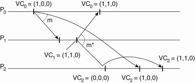
As an example, consider three processes P0, P1, and P2 as shown in Fig. 6-13. At local time (1,0,0), P1 sends message m to the other two processes. After its receipt by P1, the latter decides to send m*, which arrives at P2 sooner than m. At that point, the delivery of m* is delayed by P2 until m has been received and delivered to P2's application layer.

Figure 6-13. Enforcing causal communication.

A Note on Ordered Message Delivery

Some middleware systems, notably ISIS and its successor Horus (Birman and van Renesse, 1994), provide support for totally-ordered and causally-ordered (reliable) multicasting. There has been some controversy whether such support should be provided as part of the message-communication layer, or whether applications should handle ordering (see, e.g., Cheriton and Skeen, 1993; and Birman, 1994). Matters have not been settled, but more important is that the arguments still hold today.

There are two main problems with letting the middleware deal with message ordering. First, because the middleware cannot tell what a message actually contains, only potential causality is captured. For example, two messages from the same sender that are completely independent will always be marked as causally related by the middleware layer. This approach is overly restrictive and may lead to efficiency problems.

A second problem is that not all causality may be captured. Consider an electronic bulletin board. Suppose Alice posts an article. If she then phones Bob telling about what she just wrote, Bob may post another article as a reaction without having seen Alice's posting on the board. In other words, there is a causality between Bob's posting and that of Alice due to external communication. This causality is not captured by the bulletin board system.

[Page 252]

In essence, ordering issues, like many other application-specific communication issues, can be adequately solved by looking at the application for which communication is taking place. This is also known as the end-to-end argument in systems design (Saltzer et al., 1984). A drawback of having only application-level solutions is that a developer is forced to concentrate on issues that do not immediately relate to the core functionality of the application. For example, ordering may not be the most important problem when developing a messaging system such as an electronic bulletin board. In that case, having an underlying communication layer handle ordering may turn out to be convenient. We will come across the end-to-end argument a number of times, notably when dealing with security in distributed systems.

6.3. Mutual Exclusion

Fundamental to distributed systems is the concurrency and collaboration among multiple processes. In many cases, this also means that processes will need to simultaneously access the same resources. To prevent that such concurrent accesses corrupt the resource, or make it inconsistent, solutions are needed to grant mutual exclusive access by processes. In this section, we take a look at some of the more important distributed algorithms that have been proposed. A recent survey of distributed algorithms for mutual exclusion is provided by Saxena and Rai (2003). Older, but still relevant is Velazquez (1993).

6.3.1. Overview

Distributed mutual exclusion algorithms can be classified into two different categories. In token-based solutions mutual exclusion is achieved by passing a special message between the processes, known as a token. There is only one token available and who ever has that token is allowed to access the shared resource. When finished, the token is passed on to a next process. If a process having the token is not interested in accessing the resource, it simply passes it on.

Token-based solutions have a few important properties. First, depending on the how the processes are organized, they can fairly easily ensure that every process will get a chance at accessing the resource. In other words, they avoid starvation. Second, deadlocks by which several processes are waiting for each other to proceed, can easily be avoided, contributing to their simplicity. Unfortunately, the main drawback of token-based solutions is a rather serious one: when the token is lost (e.g., because the process holding it crashed), an intricate distributed procedure needs to be started to ensure that a new token is created, but above all, that it is also the only token.

As an alternative, many distributed mutual exclusion algorithms follow a permission-based approach. In this case, a process wanting to access the resource first requires the permission of other processes. There are many different ways toward granting such a permission and in the sections that follow we will consider a few of them.

[Page 253]

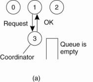
6.3.2. A Centralized Algorithm

The most straightforward way to achieve mutual exclusion in a distributed system is to simulate how it is done in a one-processor system. One process is elected as the coordinator. Whenever a process wants to access a shared resource, it sends a request message to the coordinator stating which resource it wants to access and asking for permission. If no other process is currently accessing that resource, the coordinator sends back a reply granting permission, as shown in Fig. 6-14(a). When the reply arrives, the requesting process can go ahead.

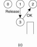
Figure 6-14. (a) Process 1 asks the coordinator for permission to access a shared resource. Permission is granted. (b) Process 2 then asks permission to access the same resource. The coordinator does not reply. (c) When process 1 releases the resource, it tells the coordinator, which then replies to 2.

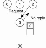
Now suppose that another process, 2 in Fig. 6-14(b), asks for permission to access the resource. The coordinator knows that a different process is already at the resource, so it cannot grant permission. The exact method used to deny permission is system dependent. In Fig. 6-14(b), the coordinator just refrains from replying, thus blocking process 2, which is waiting for a reply. Alternatively, it could send a reply saying "permission denied." Either way, it queues the request from 2 for the time being and waits for more messages.

When process 1 is finished with the resource, it sends a message to the coordinator releasing its exclusive access, as shown in Fig. 6-14(c). The coordinator takes the first item off the queue of deferred requests and sends that process a grant message. If the process was still blocked (i.e., this is the first message to it), it unblocks and accesses the resource. If an explicit message has already been sent denying permission, the process will have to poll for incoming traffic or block later. Either way, when it sees the grant, it can go ahead as well.

It is easy to see that the algorithm guarantees mutual exclusion: the coordinator only lets one process at a time to the resource. It is also fair, since requests are granted in the order in which they are received. No process ever waits forever (no starvation). The scheme is easy to implement, too, and requires only three messages per use of resource (request, grant, release). It's simplicity makes an attractive solution for many practical situations.

[Page 254]

The centralized approach also has shortcomings. The coordinator is a single point of failure, so if it crashes, the entire system may go down. If processes normally block after making a request, they cannot distinguish a dead coordinator from "permission denied" since in both cases no message comes back. In addition, in a large system, a single coordinator can become a performance bottleneck. Nevertheless, the benefits coming from its simplicity outweigh in many cases the potential drawbacks. Moreover, distributed solutions are not necessarily better, as our next example illustrates.

6.3.3. A Decentralized Algorithm

Having a single coordinator is often a poor approach. Let us take a look at fully decentralized solution. Lin et al. (2004) propose to use a voting algorithm that can be executed using a DHT-based system. In essence, their solution extends the central coordinator in the following way. Each resource is assumed to be replicated n times. Every replica has its own coordinator for controlling the access by concurrent processes.

However, whenever a process wants to access the resource, it will simply need to get a majority vote from m > n/2 coordinators. Unlike in the centralized scheme discussed before, we assume that when a coordinator does not give permission to access a resource (which it will do when it had granted permission to another process), it will tell the requester.

This scheme essentially makes the original centralized solution less vulnerable to failures of a single coordinator. The assumption is that when a coordinator crashes, it recovers quickly but will have forgotten any vote it gave before it crashed. Another way of viewing this is that a coordinator resets itself at arbitrary moments. The risk that we are taking is that a reset will make the coordinator forget that it had previously granted permission to some process to access the resource. As a consequence, it may incorrectly grant this permission again to another process after its recovery.

Let p be the probability that a coordinator resets during a time interval Δt. The probability P [k ] that k out of m coordinators reset during the same interval is then

Given that at least 2m - n coordinators need to reset in order to violate the correctness of the voting mechanism, the probability that such a violation occurs is then . To give an impression of what this could mean, assume that we are dealing with a DHT-based system in which each node participates for about 3 hours in a row. Let Δt be 10 seconds, which is considered to be a conservative value for a single process to want to access a shared resource. (Different mechanisms are needed for very long allocations.) With n = 32 and m = 0.75n, the probability of violating correctness is less than 10-40. This probability is surely smaller than the availability of any resource.

[Page 255]

To implement this scheme, Lin et al. (2004) use a DHT-based system in which a resource is replicated n times. Assume that the resource is known under its unique name rname. We can then assume that the i-th replica is named rname-i which is then used to compute a unique key using a known hash function. As a consequence, every process can generate the n keys given a resource's name, and subsequently lookup each node responsible for a replica (and controlling access to that replica).

If permission to access the resource is denied (i.e., a process gets less than m votes), it is assumed that it will back off for a randomly-chosen time, and make a next attempt later. The problem with this scheme is that if many nodes want to access the same resource, it turns out that the utilization rapidly drops. In other words, there are so many nodes competing to get access that eventually no one is able to get enough votes leaving the resource unused. A solution to solve this problem can be found in Lin et al. (2004).

6.3.4. A Distributed Algorithm

To many, having a probabilistically correct algorithm is just not good enough. So researchers have looked for deterministic distributed mutual exclusion algorithms. Lamport's 1978 paper on clock synchronization presented the first one. Ricart and Agrawala (1981) made it more efficient. In this section we will describe their method.

Ricart and Agrawala's algorithm requires that there be a total ordering of all events in the system. That is, for any pair of events, such as messages, it must be unambiguous which one actually happened first. Lamport's algorithm presented in Sec. 6.2.1 is one way to achieve this ordering and can be used to provide timestamps for distributed mutual exclusion.

The algorithm works as follows. When a process wants to access a shared resource, it builds a message containing the name of the resource, its process number, and the current (logical) time. It then sends the message to all other processes, conceptually including itself. The sending of messages is assumed to be reliable; that is, no message is lost.

When a process receives a request message from another process, the action it takes depends on its own state with respect to the resource named in the message. Three different cases have to be clearly distinguished:

[Page 256]

If the receiver is not accessing the resource and does not want to access it, it sends back an OK message to the sender.

If the receiver already has access to the resource, it simply does not reply. Instead, it queues the request.

If the receiver wants to access the resource as well but has not yet done so, it compares the timestamp of the incoming message with the one contained in the message that it has sent everyone. The lowest one wins. If the incoming message has a lower timestamp, the receiver sends back an OK message. If its own message has a lower timestamp, the receiver queues the incoming request and sends nothing.

After sending out requests asking permission, a process sits back and waits until everyone else has given permission. As soon as all the permissions are in, it may go ahead. When it is finished, it sends OK messages to all processes on its queue and deletes them all from the queue.

Let us try to understand why the algorithm works. If there is no conflict, it clearly works. However, suppose that two processes try to simultaneously access the resource, as shown in Fig. 6-15(a).

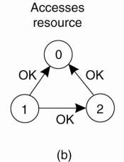
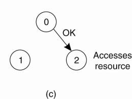
Figure 6-15. (a) Two processes want to access a shared resource at the same moment. (b) Process 0 has the lowest timestamp, so it wins. (c) When process 0 is done, it sends an OK also, so 2 can now go ahead.

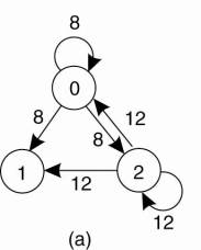
Process 0 sends everyone a request with timestamp 8, while at the same time, process 2 sends everyone a request with timestamp 12. Process 1 is not interested in the resource, so it sends OK to both senders. Processes 0 and 2 both see the conflict and compare timestamps. Process 2 sees that it has lost, so it grants permission to 0 by sending OK. Process 0 now queues the request from 2 for later processing and access the resource, as shown in Fig. 6-15(b). When it is finished, it removes the request from 2 from its queue and sends an OK message to process 2, allowing the latter to go ahead, as shown in Fig. 6-15(c). The algorithm works because in the case of a conflict, the lowest timestamp wins and everyone agrees on the ordering of the timestamps.

[Page 257]

Note that the situation in Fig. 6-15 would have been essentially different if process 2 had sent its message earlier in time so that process 0 had gotten it and granted permission before making its own request. In this case, 2 would have noticed that it itself had already access to the resource at the time of the request, and queued it instead of sending a reply.

As with the centralized algorithm discussed above, mutual exclusion is guaranteed without deadlock or starvation. The number of messages required per entry is now 2(n - 1), where the total number of processes in the system is n. Best of all, no single point of failure exists.

Unfortunately, the single point of failure has been replaced by n points of failure. If any process crashes, it will fail to respond to requests. This silence will be interpreted (incorrectly) as denial of permission, thus blocking all subsequent attempts by all processes to enter all critical regions. Since the probability of one of the n processes failing is at least n times as large as a single coordinator failing, we have managed to replace a poor algorithm with one that is more than n times worse and requires much more network traffic as well.

The algorithm can be patched up by the same trick that we proposed earlier. When a request comes in, the receiver always sends a reply, either granting or denying permission. Whenever either a request or a reply is lost, the sender times out and keeps trying until either a reply comes back or the sender concludes that the destination is dead. After a request is denied, the sender should block waiting for a subsequent OK message.

Another problem with this algorithm is that either a multicast communication primitive must be used, or each process must maintain the group membership list itself, including processes entering the group, leaving the group, and crashing. The method works best with small groups of processes that never change their group memberships.

Finally, recall that one of the problems with the centralized algorithm is that making it handle all requests can lead to a bottleneck. In the distributed algorithm, all processes are involved in all decisions concerning accessing the shared resource. If one process is unable to handle the load, it is unlikely that forcing everyone to do exactly the same thing in parallel is going to help much.

Various minor improvements are possible to this algorithm. For example, getting permission from everyone is really overkill. All that is needed is a method to prevent two processes from accessing the resource at the same time. The algorithm can be modified to grant permission when it has collected permission from a simple majority of the other processes, rather than from all of them. Of course, in this variation, after a process has granted permission to one process, it cannot grant the same permission to another process until the first one has finished.

Nevertheless, this algorithm is slower, more complicated, more expensive, and less robust that the original centralized one. Why bother studying it under these conditions? For one thing, it shows that a distributed algorithm is at least possible, something that was not obvious when we started. Also, by pointing out the shortcomings, we may stimulate future theoreticians to try to produce algorithms that are actually useful. Finally, like eating spinach and learning Latin in high school, some things are said to be good for you in some abstract way. It may take some time to discover exactly what.

6.3.5. A Token Ring Algorithm

A completely different approach to deterministically achieving mutual exclusion in a distributed system is illustrated in Fig. 6-16. Here we have a bus network, as shown in Fig. 6-16(a), (e.g., Ethernet), with no inherent ordering of the processes. In software, a logical ring is constructed in which each process is assigned a position in the ring, as shown in Fig. 6-16(b). The ring positions may be allocated in numerical order of network addresses or some other means. It does not matter what the ordering is. All that matters is that each process knows who is next in line after itself.

Figure 6-16. (a) An unordered group of processes on a network. (b) A logical ring constructed in software.

When the ring is initialized, process 0 is given a token. The token circulates around the ring. It is passed from process k to process k+1 (modulo the ring size) in point-to-point messages. When a process acquires the token from its neighbor, it checks to see if it needs to access the shared resource. If so, the process goes ahead, does all the work it needs to, and releases the resources. After it has finished, it passes the token along the ring. It is not permitted to immediately enter the resource again using the same token.

If a process is handed the token by its neighbor and is not interested in the resource, it just passes the token along. As a consequence, when no processes need the resource, the token just circulates at high speed around the ring.

The correctness of this algorithm is easy to see. Only one process has the token at any instant, so only one process can actually get to the resource. Since the token circulates among the processes in a well-defined order, starvation cannot occur. Once a process decides it wants to have access to the resource, at worst it will have to wait for every other process to use the resource.

[Page 259]

As usual, this algorithm has problems too. If the token is ever lost, it must be regenerated. In fact, detecting that it is lost is difficult, since the amount of time between successive appearances of the token on the network is unbounded. The fact that the token has not been spotted for an hour does not mean that it has been lost; somebody may still be using it.

The algorithm also runs into trouble if a process crashes, but recovery is easier than in the other cases. If we require a process receiving the token to acknowledge receipt, a dead process will be detected when its neighbor tries to give it the token and fails. At that point the dead process can be removed from the group, and the token holder can throw the token over the head of the dead process to the next member down the line, or the one after that, if necessary. Of course, doing so requires that everyone maintain the current ring configuration.

6.3.6. A Comparison of the Four Algorithms

A brief comparison of the four mutual exclusion algorithms we have looked at is instructive. In Fig. 6-17 we have listed the algorithms and three key properties: the number of messages required for a process to access and release a shared resource, the delay before access can occur (assuming messages are passed sequentially over a network), and some problems associated with each algorithm.

Figure 6-17. A comparison of three mutual exclusion algorithms.

Algorithm	Messages per entry/exit	Delay before entry (in message times)	Problems
Centralized	3	2	Coordinator crash
Decentralized	3mk, k = 1, 2,...	2 m	Starvation, low efficiency
Distributed	2(n - 1)	2(n - 1)	Crash of any process
Token ring	1 to	0 to n - 1	Lost token, process crash

The centralized algorithm is simplest and also most efficient. It requires only three messages to enter and leave a critical region: a request, a grant to enter, and a release to exit. In the decentralized case, we see that these messages need to be carried out for each of the m coordinators, but now it is possible that several attempts need to be made (for which we introduce the variable k). The distributed algorithm requires n - 1 request messages, one to each of the other processes, and an additional n - 1 grant messages, for a total of 2(n - 1). (We assume that only point-to-point communication channels are used.) With the token ring algorithm, the number is variable. If every process constantly wants to enter a critical region, then each token pass will result in one entry and exit, for an average of one message per critical region entered. At the other extreme, the token may sometimes circulate for hours without anyone being interested in it. In this case, the number of messages per entry into a critical region is unbounded.

[Page 260]

The delay from the moment a process needs to enter a critical region until its actual entry also varies for the three algorithms. When the time using a resource is short, the dominant factor in the delay is the actual mechanism for accessing a resource. When resources are used for a long time period, the dominant factor is waiting for everyone else to take their turn. In Fig. 6-17 we show the former case. It takes only two message times to enter a critical region in the centralized case, but 3mk times for the decentralized case, where k is the number of attempts that need to be made. Assuming that messages are sent one after the other, 2(n - 1) message times are needed in the distributed case. For the token ring, the time varies from 0 (token just arrived) to n - 1 (token just departed).

Finally, all algorithms except the decentralized one suffer badly in the event of crashes. Special measures and additional complexity must be introduced to avoid having a crash bring down the entire system. It is ironic that the distributed algorithms are even more sensitive to crashes than the centralized one. In a system that is designed to be fault tolerant, none of these would be suitable, but if crashes are very infrequent, they might do. The decentralized algorithm is less sensitive to crashes, but processes may suffer from starvation and special measures are needed to guarantee efficiency.

6.4. Global Positioning of Nodes

When the number of nodes in a distributed system grows, it becomes increasingly difficult for any node to keep track of the others. Such knowledge may be important for executing distributed algorithms such as routing, multicasting, data placement, searching, and so on. We have already seen different examples in which large collections of nodes are organized into specific topologies that facilitate the efficient execution of such algorithms. In this section, we take a look at another organization that is related to timing issues.

In geometric overlay networks each node is given a position in an m-dimensional geometric space, such that the distance between two nodes in that space reflects a real-world performance metric. The simplest, and most applied example, is where distance corresponds to internode latency. In other words, given two nodes P and Q, then the distance d (P,Q) reflects how long it would take for a message to travel from P to Q and vice versa.

There are many applications of geometric overlay networks. Consider the situation where a Web site at server O has been replicated to multiple servers S1,..., Sk on the Internet. When a client C requests a page from O, the latter may decide to redirect that request to the server closest to C, that is, the one that will give the best response time. If the geometric location of C is known, as well as those of each replica server, O can then simply pick that server Si for which d (C,Si) is minimal. Note that such a selection requires only local processing at O. In other words, there is, for example, no need to sample all the latencies between C and each of the replica servers.

[Page 261]

Another example, which we will work out in detail in the following chapter, is optimal replica placement. Consider again a Web site that has gathered the positions of its clients. If the site were to replicate its content to K servers, it can compute the K best positions where to place replicas such that the average client-to-replica response time is minimal. Performing such computations is almost trivially feasible if clients and servers have geometric positions that reflect internode latencies.

As a last example, consider position-based routing (Araujo and Rodrigues, 2005; and Stojmenovic, 2002). In such schemes, a message is forwarded to its destination using only positioning information. For example, a naive routing algorithm to let each node forward a message to the neighbor closest to the destination. Although it can be easily shown that this specific algorithm need not converge, it illustrates that only local information is used to take a decision. There is no need to propagate link information or such to all nodes in the network, as is the case with conventional routing algorithms.

Theoretically, positioning a node in an m-dimensional geometric space requires m+1 distance measures to nodes with known positions. This can be easily seen by considering the case m = 2, as shown in Fig. 6-18. Assuming that node P wants to compute its own position, it contacts three other nodes with known positions and measures its distance to each of them. Contacting only one node would tell P about the circle it is located on; contacting only two nodes would tell it about the position of the intersection of two circles (which generally consists of two points); a third node would subsequently allow P to compute is actual location.

[Page 262]

Figure 6-18. Computing a node's position in a two-dimensional space.

(This item is displayed on page 261 in the print version)

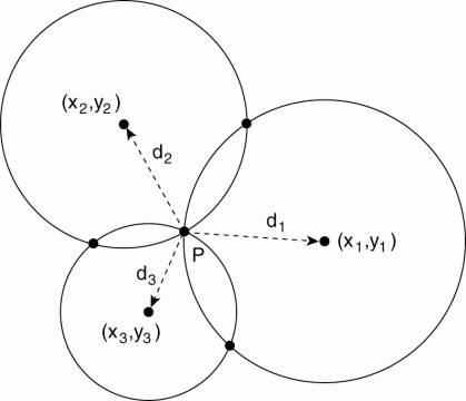
Just as in GPS, node P can compute is own coordinates (xP,yP) by solving the three equations with the two unknowns xP and yP:

As said, di generally corresponds to measuring the latency between P and the node at (xi,yi). This latency can be estimated as being half the round-trip delay, but it should be clear that its value will be different over time. The effect is a different positioning whenever P would want to recompute its position. Moreover, if other nodes would use P's current position to compute their own coordinates, then it should be clear that the error in positioning P will affect the accuracy of the positioning of other nodes.

Moreover, it should also be clear that measured distances by different nodes will generally not even be consistent. For example, assume we are computing distances in a one-dimensional space as shown in Fig. 6-19. In this example, we see that although R measures its distance to Q as 2.0, and d (P,Q) has been measured to be 1.0, when R measures d (P,R) it finds 3.2, which is clearly inconsistent with the other two measurements.

Figure 6-19. Inconsistent distance measurements in a one-dimensional space.

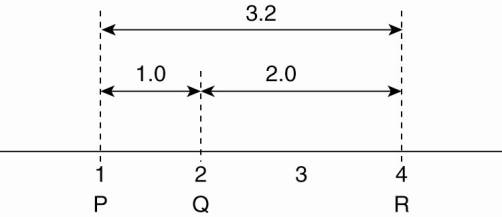
Fig. 6-19 also suggests how this situation can be improved. In our simple example, we could solve the inconsistencies by merely computing positions in a two-dimensional space. This by itself, however, is not a general solution when dealing with many measurements. In fact, considering that Internet latency measurements may violate the triangle inequality, it is generally impossible to resolve inconsistencies completely. The triangle inequality states that in a geometric space, for any arbitrary three nodes P, Q, and R it must always be true that d (P,R) d (P,Q) + d (Q,R).

There are various ways to approach these issues. One approach, proposed by Ng and Zhang (2002) is to use L special nodes b1, . . . , bL, known as landmarks. Landmarks measure their pair-wise latencies d(bi,bj) and subsequently let a central node compute the coordinates for each landmark. To this end, the central node seeks to minimize the following aggregated error function:

[Page 263]

where corresponds to the geometric distance, that is, the distance after nodes bi and bj have been positioned.

The hidden parameter in minimizing the aggregated error function is the dimension m. Obviously, we have that L > m, but nothing prevents us from choosing a value for m that is much smaller than L. In that case, a node P measures its distance to each of the L landmarks and computes its coordinates by minimizing

As it turns out, with well-chosen landmarks, m can be as small as 6 or 7, with being no more than a factor 2 different from the actual latency d (P,Q) for arbitrary nodes P and Q (Szyamniak et al., 2004).

Another way to tackle this problem is to view the collection of nodes as a huge system in which nodes are attached to each other through springs. In this case, indicates to what extent nodes P and Q are displaced relative to the situation in which the system of springs would be at rest. By letting each node (slightly) change its position, it can be shown that the system will eventually converge to an optimal organization in which the aggregated error is minimal. This approach is followed in Vivaldi, of which the details can be found in Dabek et al. (2004a).

6.5. Election Algorithms

Many distributed algorithms require one process to act as coordinator, initiator, or otherwise perform some special role. In general, it does not matter which process takes on this special responsibility, but one of them has to do it. In this section we will look at algorithms for electing a coordinator (using this as a generic name for the special process).

If all processes are exactly the same, with no distinguishing characteristics, there is no way to select one of them to be special. Consequently, we will assume that each process has a unique number, for example, its network address (for simplicity, we will assume one process per machine). In general, election algorithms attempt to locate the process with the highest process number and designate it as coordinator. The algorithms differ in the way they do the location.

[Page 264]

Furthermore, we also assume that every process knows the process number of every other process. What the processes do not know is which ones are currently up and which ones are currently down. The goal of an election algorithm is to ensure that when an election starts, it concludes with all processes agreeing on who the new coordinator is to be. There are many algorithms and variations, of which several important ones are discussed in the text books by Lynch (1996) and Tel (2000), respectively.

6.5.1. Traditional Election Algorithms

We start with taking a look at two traditional election algorithms to give an impression what whole groups of researchers have been doing in the past decades. In subsequent sections, we pay attention to new applications of the election problem.

The Bully Algorithm

As a first example, consider the bully algorithm devised by Garcia-Molina (1982). When any process notices that the coordinator is no longer responding to requests, it initiates an election. A process, P, holds an election as follows:

P sends an ELECTION message to all processes with higher numbers.

If no one responds, P wins the election and becomes coordinator.

If one of the higher-ups answers, it takes over. P's job is done.

At any moment, a process can get an ELECTION message from one of its lower-numbered colleagues. When such a message arrives, the receiver sends an OK message back to the sender to indicate that he is alive and will take over. The receiver then holds an election, unless it is already holding one. Eventually, all processes give up but one, and that one is the new coordinator. It announces its victory by sending all processes a message telling them that starting immediately it is the new coordinator.

If a process that was previously down comes back up, it holds an election. If it happens to be the highest-numbered process currently running, it will win the election and take over the coordinator's job. Thus the biggest guy in town always wins, hence the name "bully algorithm."

In Fig. 6-20 we see an example of how the bully algorithm works. The group consists of eight processes, numbered from 0 to 7. Previously process 7 was the coordinator, but it has just crashed. Process 4 is the first one to notice this, so it sends ELECTION messages to all the processes higher than it, namely 5, 6, and 7, as shown in Fig. 6-20(a). Processes 5 and 6 both respond with OK, as shown in Fig. 6-20(b). Upon getting the first of these responses, 4 knows that its job is over. It knows that one of these bigwigs will take over and become coordinator. It just sits back and waits to see who the winner will be (although at this point it can make a pretty good guess).

[Page 265]

Figure 6-20. The bully election algorithm. (a) Process 4 holds an election. (b) Processes 5 and 6 respond, telling 4 to stop. (c) Now 5 and 6 each hold an election. (d) Process 6 tells 5 to stop. (e) Process 6 wins and tells everyone.

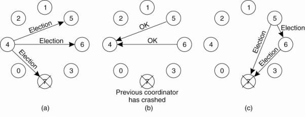
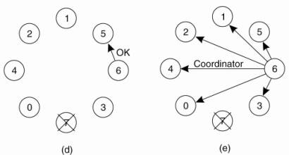
In Fig. 6-20(c), both 5 and 6 hold elections, each one only sending messages to those processes higher than itself. In Fig. 6-20(d) process 6 tells 5 that it will take over. At this point 6 knows that 7 is dead and that it (6) is the winner. If there is state information to be collected from disk or elsewhere to pick up where the old coordinator left off, 6 must now do what is needed. When it is ready to take over, 6 announces this by sending a COORDINATOR message to all running processes. When 4 gets this message, it can now continue with the operation it was trying to do when it discovered that 7 was dead, but using 6 as the coordinator this time. In this way the failure of 7 is handled and the work can continue.

If process 7 is ever restarted, it will just send all the others a COORDINATOR message and bully them into submission.

[Page 266]

A Ring Algorithm

Another election algorithm is based on the use of a ring. Unlike some ring algorithms, this one does not use a token. We assume that the processes are physically or logically ordered, so that each process knows who its successor is. When any process notices that the coordinator is not functioning, it builds an ELECTION message containing its own process number and sends the message to its successor. If the successor is down, the sender skips over the successor and goes to the next member along the ring, or the one after that, until a running process is located. At each step along the way, the sender adds its own process number to the list in the message effectively making itself a candidate to be elected as coordinator.

Eventually, the message gets back to the process that started it all. That process recognizes this event when it receives an incoming message containing its own process number. At that point, the message type is changed to COORDINATOR and circulated once again, this time to inform everyone else who the coordinator is (the list member with the highest number) and who the members of the new ring are. When this message has circulated once, it is removed and everyone goes back to work.

In Fig. 6-21 we see what happens if two processes, 2 and 5, discover simultaneously that the previous coordinator, process 7, has crashed. Each of these builds an ELECTION message and and each of them starts circulating its message, independent of the other one. Eventually, both messages will go all the way around, and both 2 and 5 will convert them into COORDINATOR messages, with exactly the same members and in the same order. When both have gone around again, both will be removed. It does no harm to have extra messages circulating; at worst it consumes a little bandwidth, but this not considered wasteful.

Figure 6-21. Election algorithm using a ring.

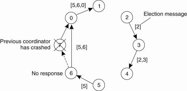
[Page 267]

6.5.2. Elections in Wireless Environments

Traditional election algorithms are generally based on assumptions that are not realistic in wireless environments. For example, they assume that message passing is reliable and that the topology of the network does not change. These assumptions are false in most wireless environments, especially those for mobile ad hoc networks.

Only few protocols for elections have been developed that work in ad hoc networks. Vasudevan et al. (2004) propose a solution that can handle failing nodes and partitioning networks. An important property of their solution is that the best leader can be elected rather than just a random as was more or less the case in the previously discussed solutions. Their protocol works as follows. To simplify our discussion, we concentrate only on ad hoc networks and ignore that nodes can move.

Consider a wireless ad hoc network. To elect a leader, any node in the network, called the source, can initiate an election by sending an ELECTION message to its immediate neighbors (i.e., the nodes in its range). When a node receives an ELECTION for the first time, it designates the sender as its parent, and subsequently sends out an ELECTION message to all its immediate neighbors, except for the parent. When a node receives an ELECTION message from a node other than its parent, it merely acknowledges the receipt.

When node R has designated node Q as its parent, it forwards the ELECTION message to its immediate neighbors (excluding Q) and waits for acknowledgments to come in before acknowledging the ELECTION message from Q. This waiting has an important consequence. First, note that neighbors that have already selected a parent will immediately respond to R. More specifically, if all neighbors already have a parent, R is a leaf node and will be able to report back to Q quickly. In doing so, it will also report information such as its battery lifetime and other resource capacities.

This information will later allow Q to compare R's capacities to that of other downstream nodes, and select the best eligible node for leadership. Of course, Q had sent an ELECTION message only because its own parent P had done so as well. In turn, when Q eventually acknowledges the ELECTION message previously sent by P, it will pass the most eligible node to P as well. In this way, the source will eventually get to know which node is best to be selected as leader, after which it will broadcast this information to all other nodes.

This process is illustrated in Fig. 6-22. Nodes have been labeled a to j, along with their capacity. Node a initiates an election by broadcasting an ELECTION message to nodes b and j, as shown in Fig. 6-22(b). After that step, ELECTION messages are propagated to all nodes, ending with the situation shown in Fig. 6-22(e), where we have omitted the last broadcast by nodes f and i. From there on, each node reports to its parent the node with the best capacity, as shown in Fig. 6-22(f). For example, when node g receives the acknowledgments from its children e and h, it will notice that h is the best node, propagating [h, 8] to its own parent, node b. In the end, the source will note that h is the best leader and will broadcast this information to all other nodes.

[Page 268]

Figure 6-22. Election algorithm in a wireless network, with node a as the source. (a) Initial network. (b)–(e) The build-tree phase (last broadcast step by nodes f and i not shown). (f)

Reporting of best node to source.

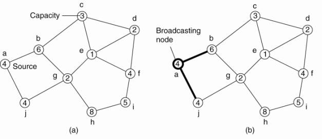
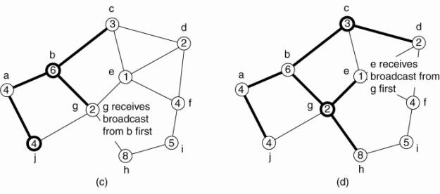
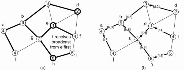
[Page 269]

When multiple elections are initiated, each node will decide to join only one election. To this end, each source tags its ELECTION message with a unique identifier. Nodes will participate only in the election with the highest identifier, stopping any running participation in other elections.

With some minor adjustments, the protocol can be shown to operate also when the network partitions, and when nodes join and leave. The details can be found in Vasudevan et al. (2004).

6.5.3. Elections in Large-Scale Systems

The algorithms we have been discussing so far generally apply to relatively small distributed systems. Moreover, the algorithms concentrate on the selection of only a single node. There are situations when several nodes should actually be selected, such as in the case of superpeers in peer-to-peer networks, which we discussed in Chap. 2. In this section, we concentrate specifically on the problem of selecting superpeers.

Lo et al. (2005) identified the following requirements that need to be met for superpeer selection:

Normal nodes should have low-latency access to superpeers.

Superpeers should be evenly distributed across the overlay network.

There should be a predefined portion of superpeers relative to the total number of nodes in the overlay network.

Each superpeer should not need to serve more than a fixed number of normal nodes.

Fortunately, these requirements are relatively easy to meet in most peer-to-peer systems, given the fact that the overlay network is either structured (as in DHT-based systems), or randomly unstructured (as, for example, can be realized with gossip-based solutions). Let us take a look at solutions proposed by Lo et al. (2005).

In the case of DHT-based systems, the basic idea is to reserve a fraction of the identifier space for superpeers. Recall that in DHT-based systems each node receives a random and uniformly assigned m-bit identifier. Now suppose we reserve the first (i.e., leftmost) k bits to identify superpeers. For example, if we need N superpeers, then the first log2(N) bits of any key can be used to identify these nodes.

To explain, assume we have a (small) Chord system with m = 8 and k = 3. When looking up the node responsible for a specific key p, we can first decide to route the lookup request to the node responsible for the pattern

p AND 11100000

[Page 270]

which is then treated as the superpeer. Note that each node id can check whether it is a superpeer by looking up

id AND 11100000

to see if this request is routed to itself. Provided node identifiers are uniformly assigned to nodes, it can be seen that with a total of N nodes the number of superpeers is, on average, equal 2k-m N.

A completely different approach is based on positioning nodes in an m-dimensional geometric space as we discussed above. In this case, assume we need to place N superpeers evenly throughout the overlay. The basic idea is simple: a total of N tokens are spread across N randomly-chosen nodes. No node can hold more than one token. Each token represents a repelling force by which another token is inclined to move away. The net effect is that if all tokens exert the same repulsion force, they will move away from each other and spread themselves evenly in the geometric space.

This approach requires that nodes holding a token learn about other tokens. To this end, Lo et al. propose to use a gossiping protocol by which a token's force is disseminated throughout the network. If a node discovers that the total forces that are acting on it exceed a threshold, it will move the token in the direction of the combined forces, as shown in Fig. 6-23.

Figure 6-23. Moving tokens in a two-dimensional space using repulsion forces.

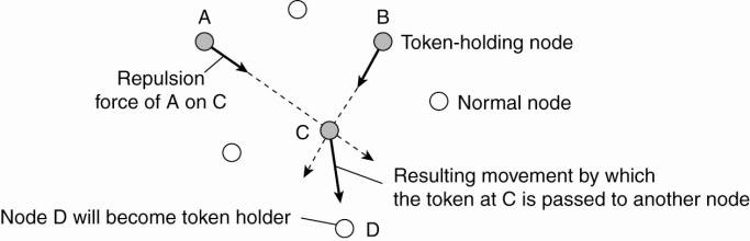
When a token is held by a node for a given amount of time, that node will promote itself to superpeer.