Introduction to Parallel Computing

Table of Contents

1. Abstract
2. Overview
   1. What is Parallel Computing?
   2. Why Use Parallel Computing?
3. Concepts and Terminology
   1. von Neumann Computer Architecture
   2. Flynn's Classical Taxonomy
   3. Some General Parallel Terminology
4. Parallel Computer Memory Architectures
   1. Shared Memory
   2. Distributed Memory
   3. Hybrid Distributed-Shared Memory
5. Parallel Programming Models
   1. Overview
   2. Shared Memory Model
   3. Threads Model
   4. Distributed Memory / Message Passing Model
   5. Data Parallel Model
   6. Hybrid Model
   7. SPMD and MPMP
6. Designing Parallel Programs
   1. Automatic vs. Manual Parallelization
   2. Understand the Problem and the Program
   3. Partitioning
   4. Communications
   5. Synchronization
   6. Data Dependencies
   7. Load Balancing
   8. Granularity
   9. I/O
   10. Limits and Costs of Parallel Programming
   11. Performance Analysis and Tuning
7. Parallel Examples
   1. Array Processing
   2. PI Calculation
   3. Simple Heat Equation
   4. 1-D Wave Equation
8. References and More Information

This tutorial is the first of eight tutorials in the 4+ day "Using LLNL's Supercomputers" workshop. It is intended to provide only a very quick overview of the extensive and broad topic of Parallel Computing, as a lead-in for the tutorials that follow it. As such, it covers just the very basics of parallel computing, and is intended for someone who is just becoming acquainted with the subject and who is planning to attend one or more of the other tutorials in this workshop. It is not intended to cover Parallel Programming in depth, as this would require significantly more time. The tutorial begins with a discussion on parallel computing - what it is and how it's used, followed by a discussion on concepts and terminology associated with parallel computing. The topics of parallel memory architectures and programming models are then explored. These topics are followed by a series of practical discussions on a number of the complex issues related to designing and running parallel programs. The tutorial concludes with several examples of how to parallelize simple serial programs.

Overview

What is Parallel Computing?

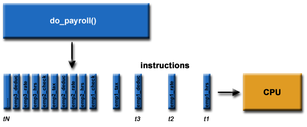
• Traditionally, software has been written for serial computation:
  • To be run on a single computer having a single Central Processing Unit (CPU);
  • A problem is broken into a discrete series of instructions.
  • Instructions are executed one after another.
  • Only one instruction may execute at any moment in time.

  

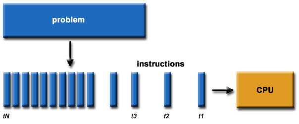
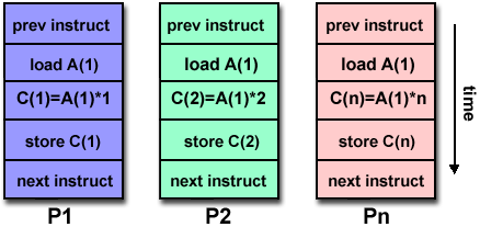
  For example:

  

• In the simplest sense, parallel computing is the simultaneous use of multiple compute resources to solve a computational problem:
  • To be run using multiple CPUs
  • A problem is broken into discrete parts that can be solved concurrently
  • Each part is further broken down to a series of instructions
  • Instructions from each part execute simultaneously on different CPUs

  

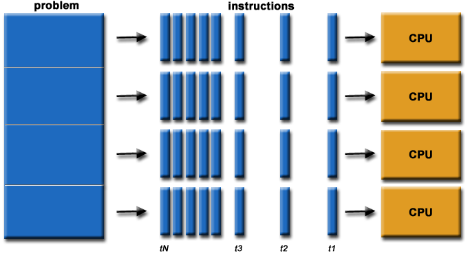
  For example:

  

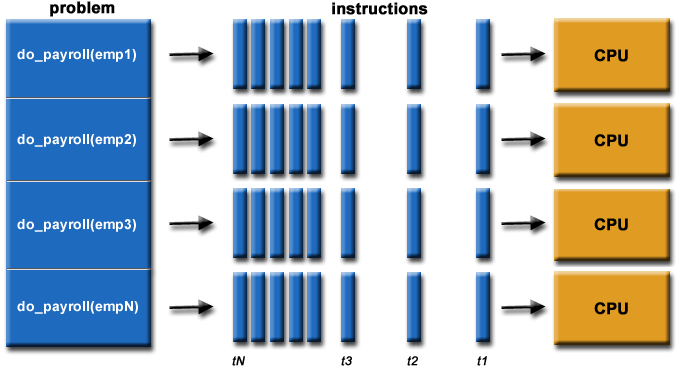
• The compute resources might be:
  • A single computer with multiple processors;
  • An arbitrary number of computers connected by a network;
  • A combination of both.

• The computational problem should be able to:
  • Be broken apart into discrete pieces of work that can be solved simultaneously;
  • Execute multiple program instructions at any moment in time;
  • Be solved in less time with multiple compute resources than with a single compute resource.

The Universe is Parallel:

• Parallel computing is an evolution of serial computing that attempts to emulate what has always been the state of affairs in the natural world: many complex, interrelated events happening at the same time, yet within a temporal sequence. For example:

  The Real World is Massively Parallel

Uses for Parallel Computing:

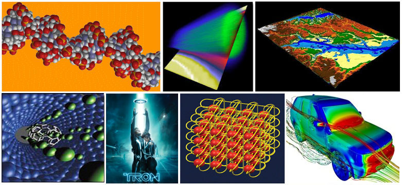
• Science and Engineering: Historically, parallel computing has been considered to be "the high end of computing", and has been used to model difficult problems in many areas of science and engineering:

  Atmosphere, Earth, Environment Physics - applied, nuclear, particle, condensed matter, high pressure, fusion, photonics Bioscience, Biotechnology, Genetics Chemistry, Molecular Sciences

  Geology, Seismology Mechanical Engineering - from prosthetics to spacecraft Electrical Engineering, Circuit Design, Microelectronics Computer Science, Mathematics

  

• Industrial and Commercial: Today, commercial applications provide an equal or greater driving force in the development of faster computers. These applications require the processing of large amounts of data in sophisticated ways. For example:

  Databases, data mining Oil exploration Web search engines, web based business services Medical imaging and diagnosis Pharmaceutical design

  Financial and economic modeling Management of national and multi-national corporations Advanced graphics and virtual reality, particularly in the entertainment industry Networked video and multi-media technologies Collaborative work environments

  

Overview

Why Use Parallel Computing?

Save time and/or money: In theory, throwing more resources at a task will shorten its time to completion, with potential cost savings. Parallel computers can be built from cheap, commodity components.
Solve larger problems: Many problems are so large and/or complex that it is impractical or impossible to solve them on a single computer, especially given limited computer memory. For example: "Grand Challenge" (en.wikipedia.org/wiki/Grand_Challenge) problems requiring PetaFLOPS and PetaBytes of computing resources. Web search engines/databases processing millions of transactions per second
Provide concurrency: A single compute resource can only do one thing at a time. Multiple computing resources can be doing many things simultaneously. For example, the Access Grid (www.accessgrid.org) provides a global collaboration network where people from around the world can meet and conduct work "virtually".
Use of non-local resources: Using compute resources on a wide area network, or even the Internet when local compute resources are scarce. For example: SETI@home (setiathome.berkeley.edu) uses over 3 million computers in over 250 countries. (June 2012) Folding@home (folding.stanford.edu) uses over 450,000 cpus globally (July 2011)
Limits to serial computing: Both physical and practical reasons pose significant constraints to simply building ever faster serial computers: Transmission speeds - the speed of a serial computer is directly dependent upon how fast data can move through hardware. Absolute limits are the speed of light (30 cm/nanosecond) and the transmission limit of copper wire (9 cm/nanosecond). Increasing speeds necessitate increasing proximity of processing elements. Limits to miniaturization - processor technology is allowing an increasing number of transistors to be placed on a chip. However, even with molecular or atomic-level components, a limit will be reached on how small components can be. Economic limitations - it is increasingly expensive to make a single processor faster. Using a larger number of moderately fast commodity processors to achieve the same (or better) performance is less expensive. Current computer architectures are increasingly relying upon hardware level parallelism to improve performance: Multiple execution units Pipelined instructions Multi-core

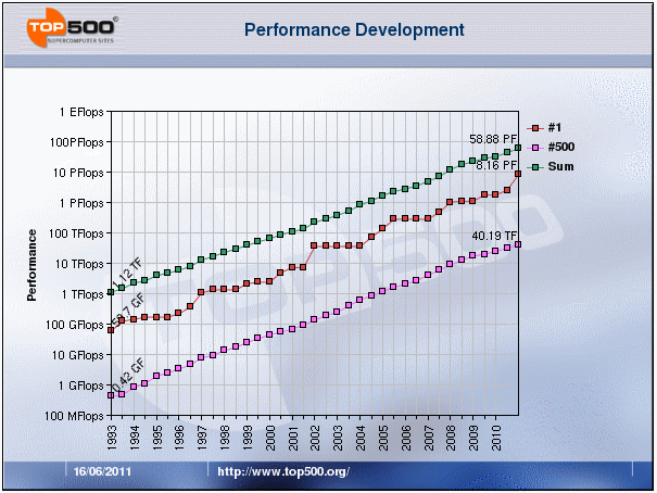
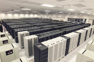
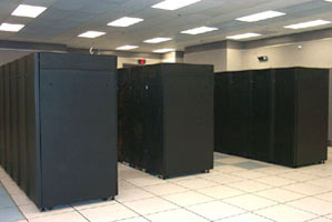
Who and What?

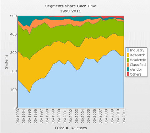
• Top500.org provides statistics on parallel computing - the charts below are just a sampling.

  

  

  

The Future:

• During the past 20+ years, the trends indicated by ever faster networks, distributed systems, and multi-processor computer architectures (even at the desktop level) clearly show that parallelism is the future of computing.

• In this same time period, there has been a greater than 1000x increase in supercomputer performance, with no end currently in sight.

• The race is already on for Exascale Computing!

Concepts and Terminology

von Neumann Architecture

• Named after the Hungarian mathematician John von Neumann who first authored the general requirements for an electronic computer in his 1945 papers.

• Since then, virtually all computers have followed this basic design, differing from earlier computers which were programmed through "hard wiring".

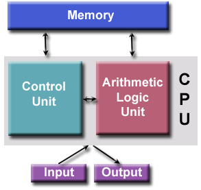  Comprised of four main components: Memory Control Unit Arithmetic Logic Unit Input/Output Read/write, random access memory is used to store both program instructions and data Program instructions are coded data which tell the computer to do something Data is simply information to be used by the program Control unit fetches instructions/data from memory, decodes the instructions and then sequentially coordinates operations to accomplish the programmed task. Aritmetic Unit performs basic arithmetic operations Input/Output is the interface to the human operator

• So what? Who cares? Well, parallel computers still follow this basic design, just multiplied in units. The basic, fundamental architecture remains the same.

Concepts and Terminology

Flynn's Classical Taxonomy

• There are different ways to classify parallel computers. One of the more widely used classifications, in use since 1966, is called Flynn's Taxonomy.

• Flynn's taxonomy distinguishes multi-processor computer architectures according to how they can be classified along the two independent dimensions of Instruction and Data. Each of these dimensions can have only one of two possible states: Single or Multiple.

• The matrix below defines the 4 possible classifications according to Flynn:

  S I S D Single Instruction, Single Data	S I M D Single Instruction, Multiple Data
  M I S D Multiple Instruction, Single Data	M I M D Multiple Instruction, Multiple Data

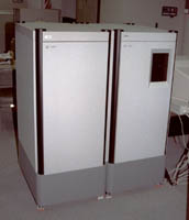
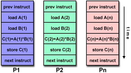
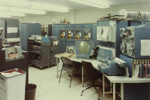
Single Instruction, Single Data (SISD): A serial (non-parallel) computer Single Instruction: Only one instruction stream is being acted on by the CPU during any one clock cycle Single Data: Only one data stream is being used as input during any one clock cycle Deterministic execution This is the oldest and even today, the most common type of computer Examples: older generation mainframes, minicomputers and workstations; most modern day PCs.

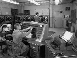
UNIVAC1	IBM 360	CRAY1
CDC 7600	PDP1	Dell Laptop

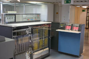
Single Instruction, Multiple Data (SIMD): A type of parallel computer Single Instruction: All processing units execute the same instruction at any given clock cycle Multiple Data: Each processing unit can operate on a different data element Best suited for specialized problems characterized by a high degree of regularity, such as graphics/image processing. Synchronous (lockstep) and deterministic execution Two varieties: Processor Arrays and Vector Pipelines Examples: Processor Arrays: Connection Machine CM-2, MasPar MP-1 & MP-2, ILLIAC IV Vector Pipelines: IBM 9000, Cray X-MP, Y-MP & C90, Fujitsu VP, NEC SX-2, Hitachi S820, ETA10 Most modern computers, particularly those with graphics processor units (GPUs) employ SIMD instructions and execution units.

ILLIAC IV

MasPar

Cray X-MP

Cray Y-MP

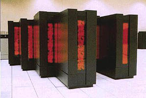
Thinking Machines CM-2

Cell Processor (GPU)

Multiple Instruction, Single Data (MISD): A type of parallel computer Multiple Instruction: Each processing unit operates on the data independently via separate instruction streams. Single Data: A single data stream is fed into multiple processing units. Few actual examples of this class of parallel computer have ever existed. One is the experimental Carnegie-Mellon C.mmp computer (1971). Some conceivable uses might be: multiple frequency filters operating on a single signal stream multiple cryptography algorithms attempting to crack a single coded message.

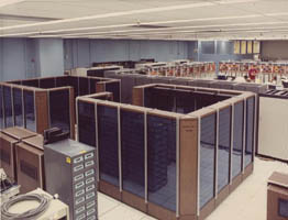
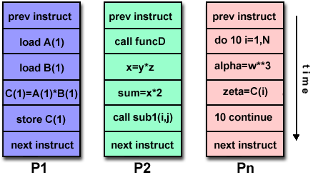
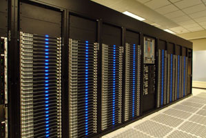
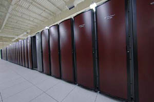
Multiple Instruction, Multiple Data (MIMD): A type of parallel computer Multiple Instruction: Every processor may be executing a different instruction stream Multiple Data: Every processor may be working with a different data stream Execution can be synchronous or asynchronous, deterministic or non-deterministic Currently, the most common type of parallel computer - most modern supercomputers fall into this category. Examples: most current supercomputers, networked parallel computer clusters and "grids", multi-processor SMP computers, multi-core PCs. Note: many MIMD architectures also include SIMD execution sub-components

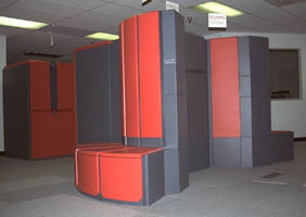
IBM POWER5

HP/Compaq Alphaserver

Intel IA32

AMD Opteron

Cray XT3

IBM BG/L

Concepts and Terminology

Some General Parallel Terminology

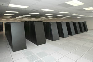
Supercomputing / High Performance Computing (HPC)

Using the world's fastest and largest computers to solve large problems.

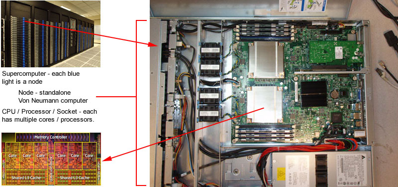
Node

A standalone "computer in a box". Usually comprised of multiple CPUs/processors/cores. Nodes are networked together to comprise a supercomputer.

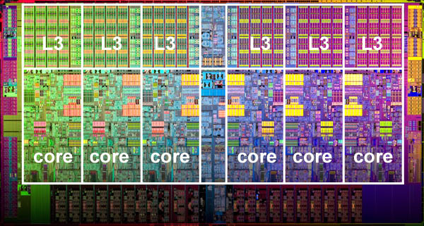
CPU / Socket / Processor / Core

This varies, depending upon who you talk to. In the past, a CPU (Central Processing Unit) was a singular execution component for a computer. Then, multiple CPUs were incorporated into a node. Then, individual CPUs were subdivided into multiple "cores", each being a unique execution unit. CPUs with multiple cores are sometimes called "sockets" - vendor dependent. The result is a node with multiple CPUs, each containing multiple cores. The nomenclature is confused at times. Wonder why?

Task

A logically discrete section of computational work. A task is typically a program or program-like set of instructions that is executed by a processor. A parallel program consists of multiple tasks running on multiple processors.

Pipelining

Breaking a task into steps performed by different processor units, with inputs streaming through, much like an assembly line; a type of parallel computing.

Shared Memory

From a strictly hardware point of view, describes a computer architecture where all processors have direct (usually bus based) access to common physical memory. In a programming sense, it describes a model where parallel tasks all have the same "picture" of memory and can directly address and access the same logical memory locations regardless of where the physical memory actually exists.

Symmetric Multi-Processor (SMP)

Hardware architecture where multiple processors share a single address space and access to all resources; shared memory computing.

Distributed Memory

In hardware, refers to network based memory access for physical memory that is not common. As a programming model, tasks can only logically "see" local machine memory and must use communications to access memory on other machines where other tasks are executing.

Communications

Parallel tasks typically need to exchange data. There are several ways this can be accomplished, such as through a shared memory bus or over a network, however the actual event of data exchange is commonly referred to as communications regardless of the method employed.

Synchronization

The coordination of parallel tasks in real time, very often associated with communications. Often implemented by establishing a synchronization point within an application where a task may not proceed further until another task(s) reaches the same or logically equivalent point.

Synchronization usually involves waiting by at least one task, and can therefore cause a parallel application's wall clock execution time to increase.

Granularity

In parallel computing, granularity is a qualitative measure of the ratio of computation to communication.

• Coarse: relatively large amounts of computational work are done between communication events
• Fine: relatively small amounts of computational work are done between communication events

Observed Speedup

Observed speedup of a code which has been parallelized, defined as:

wall-clock time of serial execution ----------------------------------- wall-clock time of parallel execution

One of the simplest and most widely used indicators for a parallel program's performance.

Parallel Overhead

The amount of time required to coordinate parallel tasks, as opposed to doing useful work. Parallel overhead can include factors such as:

• Task start-up time
• Synchronizations
• Data communications
• Software overhead imposed by parallel compilers, libraries, tools, operating system, etc.
• Task termination time

Massively Parallel

Refers to the hardware that comprises a given parallel system - having many processors. The meaning of "many" keeps increasing, but currently, the largest parallel computers can be comprised of processors numbering in the hundreds of thousands.

Embarrassingly Parallel

Solving many similar, but independent tasks simultaneously; little to no need for coordination between the tasks.

Scalability

Refers to a parallel system's (hardware and/or software) ability to demonstrate a proportionate increase in parallel speedup with the addition of more processors. Factors that contribute to scalability include:

• Hardware - particularly memory-cpu bandwidths and network communications
• Application algorithm
• Parallel overhead related
• Characteristics of your specific application and coding

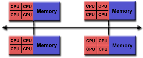
Parallel Computer Memory Architectures

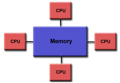
Shared Memory

Shared memory parallel computers vary widely, but generally have in common the ability for all processors to access all memory as global address space. Multiple processors can operate independently but share the same memory resources. Changes in a memory location effected by one processor are visible to all other processors. Shared memory machines can be divided into two main classes based upon memory access times: UMA and NUMA. Uniform Memory Access (UMA): Most commonly represented today by Symmetric Multiprocessor (SMP) machines Identical processors Equal access and access times to memory Sometimes called CC-UMA - Cache Coherent UMA. Cache coherent means if one processor updates a location in shared memory, all the other processors know about the update. Cache coherency is accomplished at the hardware level. 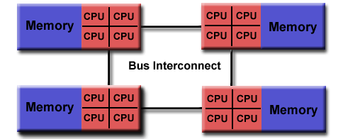Non-Uniform Memory Access (NUMA): Often made by physically linking two or more SMPs One SMP can directly access memory of another SMP Not all processors have equal access time to all memories Memory access across link is slower If cache coherency is maintained, then may also be called CC-NUMA - Cache Coherent NUMA

Shared Memory (UMA) Shared Memory (NUMA)

• Global address space provides a user-friendly programming perspective to memory
• Data sharing between tasks is both fast and uniform due to the proximity of memory to CPUs

Disadvantages:

• Primary disadvantage is the lack of scalability between memory and CPUs. Adding more CPUs can geometrically increases traffic on the shared memory-CPU path, and for cache coherent systems, geometrically increase traffic associated with cache/memory management.
• Programmer responsibility for synchronization constructs that ensure "correct" access of global memory.
• Expense: it becomes increasingly difficult and expensive to design and produce shared memory machines with ever increasing numbers of processors.

Parallel Computer Memory Architectures

Distributed Memory

• Like shared memory systems, distributed memory systems vary widely but share a common characteristic. Distributed memory systems require a communication network to connect inter-processor memory.

  

• Processors have their own local memory. Memory addresses in one processor do not map to another processor, so there is no concept of global address space across all processors.

• Because each processor has its own local memory, it operates independently. Changes it makes to its local memory have no effect on the memory of other processors. Hence, the concept of cache coherency does not apply.

• When a processor needs access to data in another processor, it is usually the task of the programmer to explicitly define how and when data is communicated. Synchronization between tasks is likewise the programmer's responsibility.

• The network "fabric" used for data transfer varies widely, though it can can be as simple as Ethernet.

Advantages:

• Memory is scalable with the number of processors. Increase the number of processors and the size of memory increases proportionately.
• Each processor can rapidly access its own memory without interference and without the overhead incurred with trying to maintain cache coherency.
• Cost effectiveness: can use commodity, off-the-shelf processors and networking.

Disadvantages:

• The programmer is responsible for many of the details associated with data communication between processors.
• It may be difficult to map existing data structures, based on global memory, to this memory organization.
• Non-uniform memory access (NUMA) times

Parallel Computer Memory Architectures

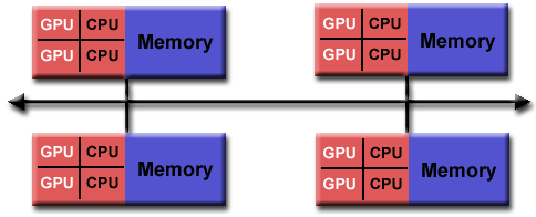
Hybrid Distributed-Shared Memory

• The largest and fastest computers in the world today employ both shared and distributed memory architectures.

• The shared memory component can be a cache coherent SMP machine and/or graphics processing units (GPU).

• The distributed memory component is the networking of multiple SMP/GPU machines, which know only about their own memory - not the memory on another machine. Therefore, network communications are required to move data from one SMP/GPU to another.

• Current trends seem to indicate that this type of memory architecture will continue to prevail and increase at the high end of computing for the foreseeable future.

• Advantages and Disadvantages: whatever is common to both shared and distributed memory architectures.

Parallel Programming Models

Overview

• There are several parallel programming models in common use:
  • Shared Memory (without threads)
  • Threads
  • Distributed Memory / Message Passing
  • Data Parallel
  • Hybrid
  • Single Program Multiple Data (SPMD)
  • Multiple Program Multiple Data (MPMD)

• Parallel programming models exist as an abstraction above hardware and memory architectures.

• Although it might not seem apparent, these models are NOT specific to a particular type of machine or memory architecture. In fact, any of these models can (theoretically) be implemented on any underlying hardware. Two examples from the past are discussed below.

  SHARED memory model on a DISTRIBUTED memory machine: Kendall Square Research (KSR) ALLCACHE approach. Machine memory was physically distributed across networked machines, but appeared to the user as a single shared memory (global address space). Generically, this approach is referred to as "virtual shared memory".

  DISTRIBUTED memory model on a SHARED memory machine: Message Passing Interface (MPI) on SGI Origin 2000. The SGI Origin 2000 employed the CC-NUMA type of shared memory architecture, where every task has direct access to global address space spread across all machines. However, the ability to send and receive messages using MPI, as is commonly done over a network of distributed memory machines, was implemented and commonly used.

• Which model to use? This is often a combination of what is available and personal choice. There is no "best" model, although there certainly are better implementations of some models over others.

• The following sections describe each of the models mentioned above, and also discuss some of their actual implementations.

Parallel Programming Models

Shared Memory Model (without threads)

• In this programming model, tasks share a common address space, which they read and write to asynchronously.

• Various mechanisms such as locks / semaphores may be used to control access to the shared memory.

• An advantage of this model from the programmer's point of view is that the notion of data "ownership" is lacking, so there is no need to specify explicitly the communication of data between tasks. Program development can often be simplified.

• An important disadvantage in terms of performance is that it becomes more difficult to understand and manage data locality.
  • Keeping data local to the processor that works on it conserves memory accesses, cache refreshes and bus traffic that occurs when multiple processors use the same data.
  • Unfortunately, controlling data locality is hard to understand and beyond the control of the average user.

Implementations:

• Native compilers and/or hardware translate user program variables into actual memory addresses, which are global. On stand-alone SMP machines, this is straightforward.

• On distributed shared memory machines, such as the SGI Origin, memory is physically distributed across a network of machines, but made global through specialized hardware and software.

Parallel Programming Models

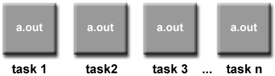
Threads Model

• This programming model is a type of shared memory programming.

• In the threads model of parallel programming, a single process can have multiple, concurrent execution paths.

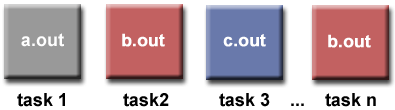
• Perhaps the most simple analogy that can be used to describe threads is the concept of a single program that includes a number of subroutines:

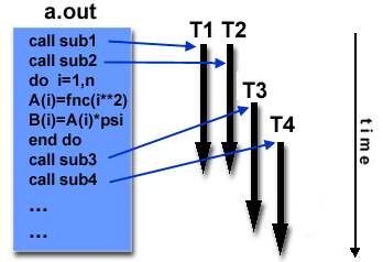
  • The main program a.out is scheduled to run by the native operating system. a.out loads and acquires all of the necessary system and user resources to run.

  • a.out performs some serial work, and then creates a number of tasks (threads) that can be scheduled and run by the operating system concurrently.

  • Each thread has local data, but also, shares the entire resources of a.out. This saves the overhead associated with replicating a program's resources for each thread. Each thread also benefits from a global memory view because it shares the memory space of a.out.

  • A thread's work may best be described as a subroutine within the main program. Any thread can execute any subroutine at the same time as other threads.

  • Threads communicate with each other through global memory (updating address locations). This requires synchronization constructs to ensure that more than one thread is not updating the same global address at any time.

  • Threads can come and go, but a.out remains present to provide the necessary shared resources until the application has completed.

Implementations:

• From a programming perspective, threads implementations commonly comprise:
  • A library of subroutines that are called from within parallel source code
  • A set of compiler directives imbedded in either serial or parallel source code

  In both cases, the programmer is responsible for determining all parallelism.

• Threaded implementations are not new in computing. Historically, hardware vendors have implemented their own proprietary versions of threads. These implementations differed substantially from each other making it difficult for programmers to develop portable threaded applications.

• Unrelated standardization efforts have resulted in two very different implementations of threads: POSIX Threads and OpenMP.

• POSIX Threads
  • Library based; requires parallel coding
  • Specified by the IEEE POSIX 1003.1c standard (1995).
  • C Language only
  • Commonly referred to as Pthreads.
  • Most hardware vendors now offer Pthreads in addition to their proprietary threads implementations.
  • Very explicit parallelism; requires significant programmer attention to detail.

• OpenMP
  • Compiler directive based; can use serial code
  • Jointly defined and endorsed by a group of major computer hardware and software vendors. The OpenMP Fortran API was released October 28, 1997. The C/C++ API was released in late 1998.
  • Portable / multi-platform, including Unix and Windows NT platforms
  • Available in C/C++ and Fortran implementations
  • Can be very easy and simple to use - provides for "incremental parallelism"

• Microsoft has its own implementation for threads, which is not related to the UNIX POSIX standard or OpenMP.

More Information:

• POSIX Threads tutorial: computing.llnl.gov/tutorials/pthreads
• OpenMP tutorial: computing.llnl.gov/tutorials/openMP

Distributed Memory / Message Passing Model

• This model demonstrates the following characteristics:

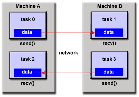
  • A set of tasks that use their own local memory during computation. Multiple tasks can reside on the same physical machine and/or across an arbitrary number of machines.

  • Tasks exchange data through communications by sending and receiving messages.

  • Data transfer usually requires cooperative operations to be performed by each process. For example, a send operation must have a matching receive operation.

Implementations:

• From a programming perspective, message passing implementations usually comprise a library of subroutines. Calls to these subroutines are imbedded in source code. The programmer is responsible for determining all parallelism.

• Historically, a variety of message passing libraries have been available since the 1980s. These implementations differed substantially from each other making it difficult for programmers to develop portable applications.

• In 1992, the MPI Forum was formed with the primary goal of establishing a standard interface for message passing implementations.

• Part 1 of the Message Passing Interface (MPI) was released in 1994. Part 2 (MPI-2) was released in 1996. Both MPI specifications are available on the web at http://www-unix.mcs.anl.gov/mpi/.

• MPI is now the "de facto" industry standard for message passing, replacing virtually all other message passing implementations used for production work. MPI implementations exist for virtually all popular parallel computing platforms. Not all implementations include everything in both MPI1 and MPI2.

More Information:

• MPI tutorial: computing.llnl.gov/tutorials/mpi

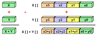
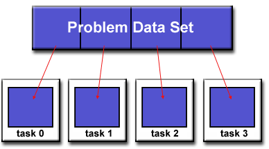
Data Parallel Model

• The data parallel model demonstrates the following characteristics:

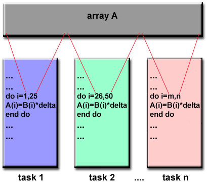
  • Most of the parallel work focuses on performing operations on a data set. The data set is typically organized into a common structure, such as an array or cube.

  • A set of tasks work collectively on the same data structure, however, each task works on a different partition of the same data structure.

  • Tasks perform the same operation on their partition of work, for example, "add 4 to every array element".

• On shared memory architectures, all tasks may have access to the data structure through global memory. On distributed memory architectures the data structure is split up and resides as "chunks" in the local memory of each task.

Implementations:

• Programming with the data parallel model is usually accomplished by writing a program with data parallel constructs. The constructs can be calls to a data parallel subroutine library or, compiler directives recognized by a data parallel compiler.

• Fortran 90 and 95 (F90, F95): ISO/ANSI standard extensions to Fortran 77.
  • Contains everything that is in Fortran 77
  • New source code format; additions to character set
  • Additions to program structure and commands
  • Variable additions - methods and arguments
  • Pointers and dynamic memory allocation added
  • Array processing (arrays treated as objects) added
  • Recursive and new intrinsic functions added
  • Many other new features

  Implementations are available for most common parallel platforms.

• High Performance Fortran (HPF): Extensions to Fortran 90 to support data parallel programming.
  • Contains everything in Fortran 90
  • Directives to tell compiler how to distribute data added
  • Assertions that can improve optimization of generated code added
  • Data parallel constructs added (now part of Fortran 95)

  HPF compilers were relatively common in the 1990s, but are no longer commonly implemented.

• Compiler Directives: Allow the programmer to specify the distribution and alignment of data. Fortran implementations are available for most common parallel platforms.

• Distributed memory implementations of this model usually require the compiler to produce object code with calls to a message passing library (MPI) for data distribution. All message passing is done invisibly to the programmer.

Hybrid Model

• A hybrid model combines more than one of the previously described programming models.

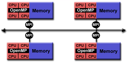
• Currently, a common example of a hybrid model is the combination of the message passing model (MPI) with the threads model (OpenMP).
  • Threads perform computationally intensive kernels using local, on-node data
  • Communications between processes on different nodes occurs over the network using MPI

• This hybrid model lends itself well to the increasingly common hardware environment of clustered multi/many-core machines.

• Another similar and increasingly popular example of a hybrid model is using MPI with GPU (Graphics Processing Unit) programming.
  • GPUs perform computationally intensive kernels using local, on-node data
  • Communications between processes on different nodes occurs over the network using MPI

SPMD and MPMD

• SPMD is actually a "high level" programming model that can be built upon any combination of the previously mentioned parallel programming models.

• SINGLE PROGRAM: All tasks execute their copy of the same program simultaneously. This program can be threads, message passing, data parallel or hybrid.

• MULTIPLE DATA: All tasks may use different data

• SPMD programs usually have the necessary logic programmed into them to allow different tasks to branch or conditionally execute only those parts of the program they are designed to execute. That is, tasks do not necessarily have to execute the entire program - perhaps only a portion of it.

• The SPMD model, using message passing or hybrid programming, is probably the most commonly used parallel programming model for multi-node clusters.

Multiple Program Multiple Data (MPMD):

• Like SPMD, MPMD is actually a "high level" programming model that can be built upon any combination of the previously mentioned parallel programming models.

• MULTIPLE PROGRAM: Tasks may execute different programs simultaneously. The programs can be threads, message passing, data parallel or hybrid.

• MULTIPLE DATA: All tasks may use different data

• MPMD applications are not as common as SPMD applications, but may be better suited for certain types of problems, particularly those that lend themselves better to functional decomposition than domain decomposition (discussed later under Partioning).

Designing Parallel Programs

Automatic vs. Manual Parallelization

• Designing and developing parallel programs has characteristically been a very manual process. The programmer is typically responsible for both identifying and actually implementing parallelism.

• Very often, manually developing parallel codes is a time consuming, complex, error-prone and iterative process.

• For a number of years now, various tools have been available to assist the programmer with converting serial programs into parallel programs. The most common type of tool used to automatically parallelize a serial program is a parallelizing compiler or pre-processor.

• A parallelizing compiler generally works in two different ways:

  • Fully Automatic
    • The compiler analyzes the source code and identifies opportunities for parallelism.
    • The analysis includes identifying inhibitors to parallelism and possibly a cost weighting on whether or not the parallelism would actually improve performance.
    • Loops (do, for) loops are the most frequent target for automatic parallelization.

  • Programmer Directed
    • Using "compiler directives" or possibly compiler flags, the programmer explicitly tells the compiler how to parallelize the code.
    • May be able to be used in conjunction with some degree of automatic parallelization also.

• If you are beginning with an existing serial code and have time or budget constraints, then automatic parallelization may be the answer. However, there are several important caveats that apply to automatic parallelization:
  • Wrong results may be produced
  • Performance may actually degrade
  • Much less flexible than manual parallelization
  • Limited to a subset (mostly loops) of code
  • May actually not parallelize code if the analysis suggests there are inhibitors or the code is too complex

• The remainder of this section applies to the manual method of developing parallel codes.

Designing Parallel Programs

Understand the Problem and the Program

• Undoubtedly, the first step in developing parallel software is to first understand the problem that you wish to solve in parallel. If you are starting with a serial program, this necessitates understanding the existing code also.

• Before spending time in an attempt to develop a parallel solution for a problem, determine whether or not the problem is one that can actually be parallelized.

  • Example of Parallelizable Problem:

    Calculate the potential energy for each of several thousand independent conformations of a molecule. When done, find the minimum energy conformation.

    This problem is able to be solved in parallel. Each of the molecular conformations is independently determinable. The calculation of the minimum energy conformation is also a parallelizable problem.

  • Example of a Non-parallelizable Problem:

    Calculation of the Fibonacci series (0,1,1,2,3,5,8,13,21,...) by use of the formula: F(n) = F(n-1) + F(n-2)

    This is a non-parallelizable problem because the calculation of the Fibonacci sequence as shown would entail dependent calculations rather than independent ones. The calculation of the F(n) value uses those of both F(n-1) and F(n-2). These three terms cannot be calculated independently and therefore, not in parallel.

Identify the program's hotspots: Know where most of the real work is being done. The majority of scientific and technical programs usually accomplish most of their work in a few places. Profilers and performance analysis tools can help here Focus on parallelizing the hotspots and ignore those sections of the program that account for little CPU usage. Identify bottlenecks in the program Are there areas that are disproportionately slow, or cause parallelizable work to halt or be deferred? For example, I/O is usually something that slows a program down. May be possible to restructure the program or use a different algorithm to reduce or eliminate unnecessary slow areas Identify inhibitors to parallelism. One common class of inhibitor is data dependence, as demonstrated by the Fibonacci sequence above. Investigate other algorithms if possible. This may be the single most important consideration when designing a parallel application.

Designing Parallel Programs

Partitioning

• One of the first steps in designing a parallel program is to break the problem into discrete "chunks" of work that can be distributed to multiple tasks. This is known as decomposition or partitioning.

• There are two basic ways to partition computational work among parallel tasks: domain decomposition and functional decomposition.

Domain Decomposition:

• In this type of partitioning, the data associated with a problem is decomposed. Each parallel task then works on a portion of of the data.

  

• There are different ways to partition data:

  

Functional Decomposition:

• In this approach, the focus is on the computation that is to be performed rather than on the data manipulated by the computation. The problem is decomposed according to the work that must be done. Each task then performs a portion of the overall work.

  

• Functional decomposition lends itself well to problems that can be split into different tasks. For example:

  Ecosystem Modeling
  Each program calculates the population of a given group, where each group's growth depends on that of its neighbors. As time progresses, each process calculates its current state, then exchanges information with the neighbor populations. All tasks then progress to calculate the state at the next time step.

  

  Signal Processing
  An audio signal data set is passed through four distinct computational filters. Each filter is a separate process. The first segment of data must pass through the first filter before progressing to the second. When it does, the second segment of data passes through the first filter. By the time the fourth segment of data is in the first filter, all four tasks are busy.

  

  Climate Modeling
  Each model component can be thought of as a separate task. Arrows represent exchanges of data between components during computation: the atmosphere model generates wind velocity data that are used by the ocean model, the ocean model generates sea surface temperature data that are used by the atmosphere model, and so on.

  

• Combining these two types of problem decomposition is common and natural.

Communications

The need for communications between tasks depends upon your problem:

• You DON'T need communications
  • Some types of problems can be decomposed and executed in parallel with virtually no need for tasks to share data. For example, imagine an image processing operation where every pixel in a black and white image needs to have its color reversed. The image data can easily be distributed to multiple tasks that then act independently of each other to do their portion of the work.
  • These types of problems are often called embarrassingly parallel because they are so straight-forward. Very little inter-task communication is required.

• You DO need communications
  • Most parallel applications are not quite so simple, and do require tasks to share data with each other. For example, a 3-D heat diffusion problem requires a task to know the temperatures calculated by the tasks that have neighboring data. Changes to neighboring data has a direct effect on that task's data.

Factors to Consider:

There are a number of important factors to consider when designing your program's inter-task communications:

• Cost of communications
  • Inter-task communication virtually always implies overhead.
  • Machine cycles and resources that could be used for computation are instead used to package and transmit data.
  • Communications frequently require some type of synchronization between tasks, which can result in tasks spending time "waiting" instead of doing work.
  • Competing communication traffic can saturate the available network bandwidth, further aggravating performance problems.

• Latency vs. Bandwidth
  • latency is the time it takes to send a minimal (0 byte) message from point A to point B. Commonly expressed as microseconds.
  • bandwidth is the amount of data that can be communicated per unit of time. Commonly expressed as megabytes/sec or gigabytes/sec.
  • Sending many small messages can cause latency to dominate communication overheads. Often it is more efficient to package small messages into a larger message, thus increasing the effective communications bandwidth.

• Visibility of communications
  • With the Message Passing Model, communications are explicit and generally quite visible and under the control of the programmer.
  • With the Data Parallel Model, communications often occur transparently to the programmer, particularly on distributed memory architectures. The programmer may not even be able to know exactly how inter-task communications are being accomplished.

• Synchronous vs. asynchronous communications
  • Synchronous communications require some type of "handshaking" between tasks that are sharing data. This can be explicitly structured in code by the programmer, or it may happen at a lower level unknown to the programmer.
  • Synchronous communications are often referred to as blocking communications since other work must wait until the communications have completed.
  • Asynchronous communications allow tasks to transfer data independently from one another. For example, task 1 can prepare and send a message to task 2, and then immediately begin doing other work. When task 2 actually receives the data doesn't matter.
  • Asynchronous communications are often referred to as non-blocking communications since other work can be done while the communications are taking place.
  • Interleaving computation with communication is the single greatest benefit for using asynchronous communications.

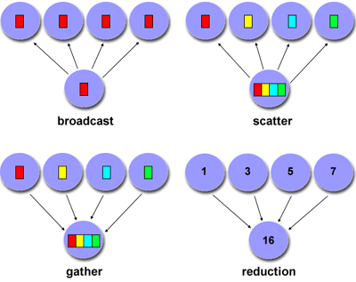
• Scope of communications
  • Knowing which tasks must communicate with each other is critical during the design stage of a parallel code. Both of the two scopings described below can be implemented synchronously or asynchronously.
  • Point-to-point - involves two tasks with one task acting as the sender/producer of data, and the other acting as the receiver/consumer.
  • Collective - involves data sharing between more than two tasks, which are often specified as being members in a common group, or collective. Some common variations (there are more):

    

• Efficiency of communications
  • Very often, the programmer will have a choice with regard to factors that can affect communications performance. Only a few are mentioned here.
  • Which implementation for a given model should be used? Using the Message Passing Model as an example, one MPI implementation may be faster on a given hardware platform than another.
  • What type of communication operations should be used? As mentioned previously, asynchronous communication operations can improve overall program performance.
  • Network media - some platforms may offer more than one network for communications. Which one is best?

• Overhead and Complexity

  

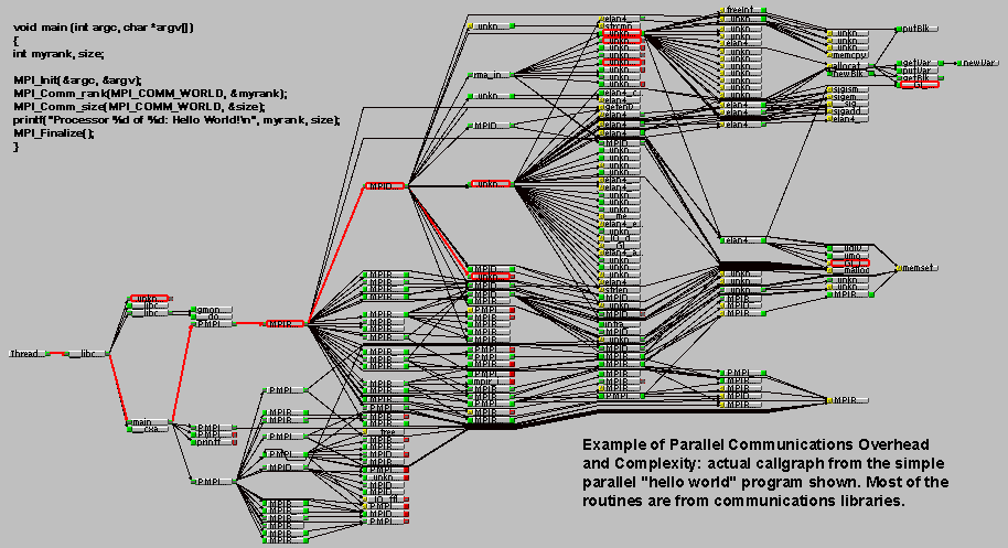
• Finally, realize that this is only a partial list of things to consider!!!

Designing Parallel Programs

Synchronization

• Barrier
  • Usually implies that all tasks are involved
  • Each task performs its work until it reaches the barrier. It then stops, or "blocks".
  • When the last task reaches the barrier, all tasks are synchronized.
  • What happens from here varies. Often, a serial section of work must be done. In other cases, the tasks are automatically released to continue their work.

• Lock / semaphore
  • Can involve any number of tasks
  • Typically used to serialize (protect) access to global data or a section of code. Only one task at a time may use (own) the lock / semaphore / flag.
  • The first task to acquire the lock "sets" it. This task can then safely (serially) access the protected data or code.
  • Other tasks can attempt to acquire the lock but must wait until the task that owns the lock releases it.
  • Can be blocking or non-blocking

• Synchronous communication operations
  • Involves only those tasks executing a communication operation
  • When a task performs a communication operation, some form of coordination is required with the other task(s) participating in the communication. For example, before a task can perform a send operation, it must first receive an acknowledgment from the receiving task that it is OK to send.
  • Discussed previously in the Communications section.

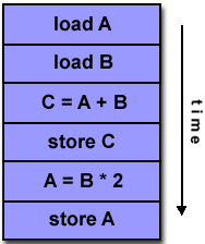
Designing Parallel Programs

Data Dependencies

• A dependence exists between program statements when the order of statement execution affects the results of the program.

• A data dependence results from multiple use of the same location(s) in storage by different tasks.

• Dependencies are important to parallel programming because they are one of the primary inhibitors to parallelism.

Examples:

• Loop carried data dependence

  DO 500 J = MYSTART,MYEND A(J) = A(J-1) * 2.0 500 CONTINUE

  The value of A(J-1) must be computed before the value of A(J), therefore A(J) exhibits a data dependency on A(J-1). Parallelism is inhibited.

  If Task 2 has A(J) and task 1 has A(J-1), computing the correct value of A(J) necessitates:

  • Distributed memory architecture - task 2 must obtain the value of A(J-1) from task 1 after task 1 finishes its computation
  • Shared memory architecture - task 2 must read A(J-1) after task 1 updates it

• Loop independent data dependence

  task 1 task 2 ------ ------ X = 2 X = 4 . . . . Y = X**2 Y = X**3

  As with the previous example, parallelism is inhibited. The value of Y is dependent on:

  • Distributed memory architecture - if or when the value of X is communicated between the tasks.
  • Shared memory architecture - which task last stores the value of X.

• Although all data dependencies are important to identify when designing parallel programs, loop carried dependencies are particularly important since loops are possibly the most common target of parallelization efforts.

How to Handle Data Dependencies:

• Distributed memory architectures - communicate required data at synchronization points.

• Shared memory architectures -synchronize read/write operations between tasks.

Designing Parallel Programs

Load Balancing

• Load balancing refers to the practice of distributing work among tasks so that all tasks are kept busy all of the time. It can be considered a minimization of task idle time.

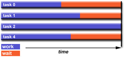
• Load balancing is important to parallel programs for performance reasons. For example, if all tasks are subject to a barrier synchronization point, the slowest task will determine the overall performance.

  

• Equally partition the work each task receives
  • For array/matrix operations where each task performs similar work, evenly distribute the data set among the tasks.
  • For loop iterations where the work done in each iteration is similar, evenly distribute the iterations across the tasks.
  • If a heterogeneous mix of machines with varying performance characteristics are being used, be sure to use some type of performance analysis tool to detect any load imbalances. Adjust work accordingly.

• Use dynamic work assignment
  • Certain classes of problems result in load imbalances even if data is evenly distributed among tasks:
    • Sparse arrays - some tasks will have actual data to work on while others have mostly "zeros".
    • Adaptive grid methods - some tasks may need to refine their mesh while others don't.
    • N-body simulations - where some particles may migrate to/from their original task domain to another task's; where the particles owned by some tasks require more work than those owned by other tasks.
  • When the amount of work each task will perform is intentionally variable, or is unable to be predicted, it may be helpful to use a scheduler - task pool approach. As each task finishes its work, it queues to get a new piece of work.
  • It may become necessary to design an algorithm which detects and handles load imbalances as they occur dynamically within the code.

Designing Parallel Programs

Granularity

• In parallel computing, granularity is a qualitative measure of the ratio of computation to communication.

• Periods of computation are typically separated from periods of communication by synchronization events.

Fine-grain Parallelism: Relatively small amounts of computational work are done between communication events Low computation to communication ratio Facilitates load balancing Implies high communication overhead and less opportunity for performance enhancement If granularity is too fine it is possible that the overhead required for communications and synchronization between tasks takes longer than the computation. 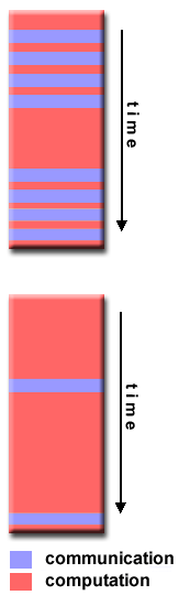Coarse-grain Parallelism: Relatively large amounts of computational work are done between communication/synchronization events High computation to communication ratio Implies more opportunity for performance increase Harder to load balance efficiently Which is Best? The most efficient granularity is dependent on the algorithm and the hardware environment in which it runs. In most cases the overhead associated with communications and synchronization is high relative to execution speed so it is advantageous to have coarse granularity. Fine-grain parallelism can help reduce overheads due to load imbalance.

Designing Parallel Programs

I/O

• I/O operations are generally regarded as inhibitors to parallelism

• Parallel I/O systems may be immature or not available for all platforms

• In an environment where all tasks see the same file space, write operations can result in file overwriting

• Read operations can be affected by the file server's ability to handle multiple read requests at the same time

• I/O that must be conducted over the network (NFS, non-local) can cause severe bottlenecks and even crash file servers.

The Good News:

• Parallel file systems are available. For example:
  • GPFS: General Parallel File System for AIX (IBM)
  • Lustre: for Linux clusters (Oracle)
  • PVFS/PVFS2: Parallel Virtual File System for Linux clusters (Clemson/Argonne/Ohio State/others)
  • PanFS: Panasas ActiveScale File System for Linux clusters (Panasas, Inc.)
  • HP SFS: HP StorageWorks Scalable File Share. Lustre based parallel file system (Global File System for Linux) product from HP

• The parallel I/O programming interface specification for MPI has been available since 1996 as part of MPI-2. Vendor and "free" implementations are now commonly available.

• A few pointers:

  • Rule #1: Reduce overall I/O as much as possible

  • If you have access to a parallel file system, investigate using it.

  • Writing large chunks of data rather than small packets is usually significantly more efficient.

  • Confine I/O to specific serial portions of the job, and then use parallel communications to distribute data to parallel tasks. For example, Task 1 could read an input file and then communicate required data to other tasks. Likewise, Task 1 could perform write operation after receiving required data from all other tasks.

  • Use local, on-node file space for I/O if possible. For example, each node may have /tmp filespace which can used. This is usually much more efficient than performing I/O over the network to one's home directory.

Designing Parallel Programs

Limits and Costs of Parallel Programming

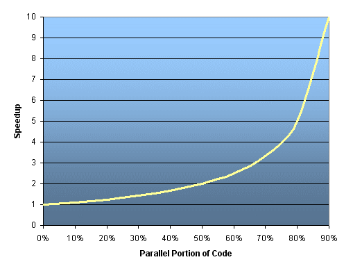
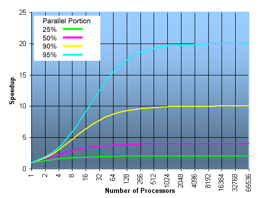
Amdahl's Law states that potential program speedup is defined by the fraction of code (P) that can be parallelized: 1 speedup = -------- 1 - P If none of the code can be parallelized, P = 0 and the speedup = 1 (no speedup). If all of the code is parallelized, P = 1 and the speedup is infinite (in theory). If 50% of the code can be parallelized, maximum speedup = 2, meaning the code will run twice as fast. Introducing the number of processors performing the parallel fraction of work, the relationship can be modeled by: 1 speedup = ------------ P + S --- N where P = parallel fraction, N = number of processors and S = serial fraction. It soon becomes obvious that there are limits to the scalability of parallelism. For example: speedup -------------------------------- N P = .50 P = .90 P = .99 ----- ------- ------- ------- 10 1.82 5.26 9.17 100 1.98 9.17 50.25 1000 1.99 9.91 90.99 10000 1.99 9.91 99.02 100000 1.99 9.99 99.90

• However, certain problems demonstrate increased performance by increasing the problem size. For example:

  
      2D Grid Calculations     85 seconds   85%
      Serial fraction          15 seconds   15%
  

  We can increase the problem size by doubling the grid dimensions and halving the time step. This results in four times the number of grid points and twice the number of time steps. The timings then look like:

  
      2D Grid Calculations     680 seconds   97.84%
      Serial fraction           15 seconds    2.16%
  

• Problems that increase the percentage of parallel time with their size are more scalable than problems with a fixed percentage of parallel time.

Complexity:

• In general, parallel applications are much more complex than corresponding serial applications, perhaps an order of magnitude. Not only do you have multiple instruction streams executing at the same time, but you also have data flowing between them.

• The costs of complexity are measured in programmer time in virtually every aspect of the software development cycle:
  • Design
  • Coding
  • Debugging
  • Tuning
  • Maintenance

• Adhering to "good" software development practices is essential when when working with parallel applications - especially if somebody besides you will have to work with the software.

Portability:

• Thanks to standardization in several APIs, such as MPI, POSIX threads, HPF and OpenMP, portability issues with parallel programs are not as serious as in years past. However...

• All of the usual portability issues associated with serial programs apply to parallel programs. For example, if you use vendor "enhancements" to Fortran, C or C++, portability will be a problem.

• Even though standards exist for several APIs, implementations will differ in a number of details, sometimes to the point of requiring code modifications in order to effect portability.

• Operating systems can play a key role in code portability issues.

• Hardware architectures are characteristically highly variable and can affect portability.

Resource Requirements:

• The primary intent of parallel programming is to decrease execution wall clock time, however in order to accomplish this, more CPU time is required. For example, a parallel code that runs in 1 hour on 8 processors actually uses 8 hours of CPU time.

• The amount of memory required can be greater for parallel codes than serial codes, due to the need to replicate data and for overheads associated with parallel support libraries and subsystems.

• For short running parallel programs, there can actually be a decrease in performance compared to a similar serial implementation. The overhead costs associated with setting up the parallel environment, task creation, communications and task termination can comprise a significant portion of the total execution time for short runs.

Scalability:

• The ability of a parallel program's performance to scale is a result of a number of interrelated factors. Simply adding more machines is rarely the answer.

• The algorithm may have inherent limits to scalability. At some point, adding more resources causes performance to decrease. Most parallel solutions demonstrate this characteristic at some point.

• Hardware factors play a significant role in scalability. Examples:
  • Memory-cpu bus bandwidth on an SMP machine
  • Communications network bandwidth
  • Amount of memory available on any given machine or set of machines
  • Processor clock speed

• Parallel support libraries and subsystems software can limit scalability independent of your application.

Designing Parallel Programs

Performance Analysis and Tuning

• As with debugging, monitoring and analyzing parallel program execution is significantly more of a challenge than for serial programs.

• A number of parallel tools for execution monitoring and program analysis are available.

• Some are quite useful; some are cross-platform also.

• Some starting points:
  • LC's "Supported Software and Computing Tools" web pages at: computing.llnl.gov/code/content/software_tools.php
  • A dated, but potentially useful LC whitepaper on the subject of "High Performance Tools and Technologies" describes a large number of tools, and a number of performance related topics applicable to code developers. Find it at: computing.llnl.gov/tutorials/performance_tools/HighPerformanceToolsTechnologiesLC.pdf.
  • Performance Analysis Tools Tutorial

• Work remains to be done, particularly in the area of scalability.

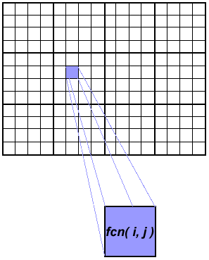
Array Processing

This example demonstrates calculations on 2-dimensional array elements, with the computation on each array element being independent from other array elements. The serial program calculates one element at a time in sequential order. Serial code could be of the form: do j = 1,n do i = 1,n a(i,j) = fcn(i,j) end do end do The calculation of elements is independent of one another - leads to an embarrassingly parallel situation. The problem should be computationally intensive.

Array Processing
Parallel Solution 1

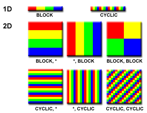
Arrays elements are distributed so that each processor owns a portion of an array (subarray). Independent calculation of array elements ensures there is no need for communication between tasks. Distribution scheme is chosen by other criteria, e.g. unit stride (stride of 1) through the subarrays. Unit stride maximizes cache/memory usage. Since it is desirable to have unit stride through the subarrays, the choice of a distribution scheme depends on the programming language. See the Block - Cyclic Distributions Diagram for the options. After the array is distributed, each task executes the portion of the loop corresponding to the data it owns. For example, with Fortran block distribution: do j = mystart, myend do i = 1,n a(i,j) = fcn(i,j) end do end do Notice that only the outer loop variables are different from the serial solution.

One Possible Solution:

• Implement as a Single Program Multiple Data (SPMD) model.

• Master process initializes array, sends info to worker processes and receives results.

• Worker process receives info, performs its share of computation and sends results to master.

• Using the Fortran storage scheme, perform block distribution of the array.

• Pseudo code solution: red highlights changes for parallelism.

  find out if I am MASTER or WORKER if I am MASTER initialize the array send each WORKER info on part of array it owns send each WORKER its portion of initial array receive from each WORKER results else if I am WORKER receive from MASTER info on part of array I own receive from MASTER my portion of initial array # calculate my portion of array do j = my first column,my last column do i = 1,n a(i,j) = fcn(i,j) end do end do send MASTER results endif

• Example MPI Program in C:   mpi_array.c

• Example MPI Program in Fortran:   mpi_array.f

Array Processing
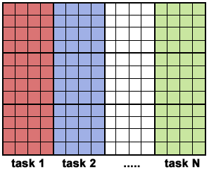
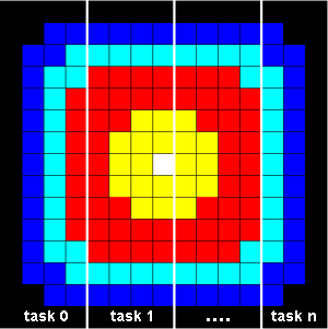
Parallel Solution 2: Pool of Tasks

• The previous array solution demonstrated static load balancing:
  • Each task has a fixed amount of work to do
  • May be significant idle time for faster or more lightly loaded processors - slowest tasks determines overall performance.

• Static load balancing is not usually a major concern if all tasks are performing the same amount of work on identical machines.

• If you have a load balance problem (some tasks work faster than others), you may benefit by using a "pool of tasks" scheme.

Pool of Tasks Scheme:

• Two processes are employed

  Master Process:

  • Holds pool of tasks for worker processes to do
  • Sends worker a task when requested
  • Collects results from workers

  Worker Process: repeatedly does the following

  • Gets task from master process
  • Performs computation
  • Sends results to master

• Worker processes do not know before runtime which portion of array they will handle or how many tasks they will perform.

• Dynamic load balancing occurs at run time: the faster tasks will get more work to do.

• Pseudo code solution: red highlights changes for parallelism.

  find out if I am MASTER or WORKER if I am MASTER do until no more jobs if request send to WORKER next job else receive results from WORKER end do else if I am WORKER do until no more jobs request job from MASTER receive from MASTER next job calculate array element: a(i,j) = fcn(i,j) send results to MASTER end do endif

Discussion:

• In the above pool of tasks example, each task calculated an individual array element as a job. The computation to communication ratio is finely granular.

• Finely granular solutions incur more communication overhead in order to reduce task idle time.

• A more optimal solution might be to distribute more work with each job. The "right" amount of work is problem dependent.

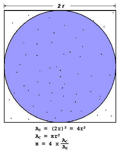
PI Calculation

The value of PI can be calculated in a number of ways. Consider the following method of approximating PI Inscribe a circle in a square Randomly generate points in the square Determine the number of points in the square that are also in the circle Let r be the number of points in the circle divided by the number of points in the square PI ~ 4 r Note that the more points generated, the better the approximation Serial pseudo code for this procedure: npoints = 10000 circle_count = 0 do j = 1,npoints generate 2 random numbers between 0 and 1 xcoordinate = random1 ycoordinate = random2 if (xcoordinate, ycoordinate) inside circle then circle_count = circle_count + 1 end do PI = 4.0*circle_count/npoints Note that most of the time in running this program would be spent executing the loop Leads to an embarrassingly parallel solution Computationally intensive Minimal communication Minimal I/O

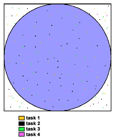
PI Calculation
Parallel Solution

Parallel strategy: break the loop into portions that can be executed by the tasks. For the task of approximating PI: Each task executes its portion of the loop a number of times. Each task can do its work without requiring any information from the other tasks (there are no data dependencies). Uses the SPMD model. One task acts as master and collects the results. Pseudo code solution: red highlights changes for parallelism. npoints = 10000 circle_count = 0 p = number of tasks num = npoints/p find out if I am MASTER or WORKER do j = 1,num generate 2 random numbers between 0 and 1 xcoordinate = random1 ycoordinate = random2 if (xcoordinate, ycoordinate) inside circle then circle_count = circle_count + 1 end do if I am MASTER receive from WORKERS their circle_counts compute PI (use MASTER and WORKER calculations) else if I am WORKER send to MASTER circle_count endif

• Example MPI Program in C:   mpi_pi_reduce.c     dboard.c

• Example MPI Program in Fortran:   mpi_pi_reduce.f     dboard.f

Simple Heat Equation

Most problems in parallel computing require communication among the tasks. A number of common problems require communication with "neighbor" tasks. The heat equation describes the temperature change over time, given initial temperature distribution and boundary conditions. A finite differencing scheme is employed to solve the heat equation numerically on a square region. The initial temperature is zero on the boundaries and high in the middle. The boundary temperature is held at zero. For the fully explicit problem, a time stepping algorithm is used. The elements of a 2-dimensional array represent the temperature at points on the square. The calculation of an element is dependent upon neighbor element values. 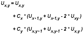A serial program would contain code like: do iy = 2, ny - 1 do ix = 2, nx - 1 u2(ix, iy) = u1(ix, iy) + cx * (u1(ix+1,iy) + u1(ix-1,iy) - 2.*u1(ix,iy)) + cy * (u1(ix,iy+1) + u1(ix,iy-1) - 2.*u1(ix,iy)) end do end do

Simple Heat Equation
Parallel Solution

• Implement as an SPMD model

• The entire array is partitioned and distributed as subarrays to all tasks. Each task owns a portion of the total array.

• Determine data dependencies
  • interior elements belonging to a task are independent of other tasks
  • border elements are dependent upon a neighbor task's data, necessitating communication.

• Master process sends initial info to workers, and then waits to collect results from all workers

• Worker process calculates solution within specified number of time steps, communicating as necessary with neighbor processes

• Pseudo code solution: red highlights changes for parallelism.

  find out if I am MASTER or WORKER if I am MASTER initialize array send each WORKER starting info and subarray receive results from each WORKER else if I am WORKER receive from MASTER starting info and subarray do t = 1, nsteps update time send neighbors my border info receive from neighbors their border info update my portion of solution array end do send MASTER results endif

• Example MPI Program in C:   mpi_heat2D.c

• Example MPI Program in Fortran:   mpi_heat2D.f

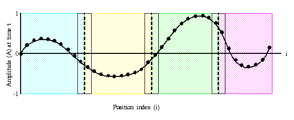
1-D Wave Equation

• In this example, the amplitude along a uniform, vibrating string is calculated after a specified amount of time has elapsed.

• The calculation involves:
  • the amplitude on the y axis
  • i as the position index along the x axis
  • node points imposed along the string
  • update of the amplitude at discrete time steps.

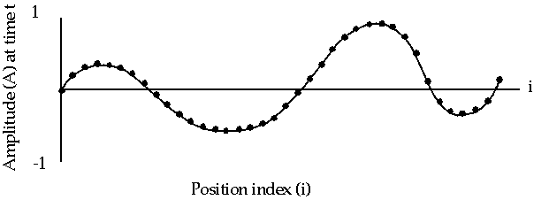
• The equation to be solved is the one-dimensional wave equation:

  
      A(i,t+1) = (2.0 * A(i,t)) - A(i,t-1) 
          + (c * (A(i-1,t) - (2.0 * A(i,t)) + A(i+1,t))) 
      

  where c is a constant

• Note that amplitude will depend on previous timesteps (t, t-1) and neighboring points (i-1, i+1). Data dependence will mean that a parallel solution will involve communications.

1-D Wave Equation
Parallel Solution

• Implement as an SPMD model

• The entire amplitude array is partitioned and distributed as subarrays to all tasks. Each task owns a portion of the total array.

• Load balancing: all points require equal work, so the points should be divided equally

• A block decomposition would have the work partitioned into the number of tasks as chunks, allowing each task to own mostly contiguous data points.

• Communication need only occur on data borders. The larger the block size the less the communication.

• Pseudo code solution:

  find out number of tasks and task identities #Identify left and right neighbors left_neighbor = mytaskid - 1 right_neighbor = mytaskid +1 if mytaskid = first then left_neigbor = last if mytaskid = last then right_neighbor = first find out if I am MASTER or WORKER if I am MASTER initialize array send each WORKER starting info and subarray else if I am WORKER` receive starting info and subarray from MASTER endif #Update values for each point along string #In this example the master participates in calculations do t = 1, nsteps send left endpoint to left neighbor receive left endpoint from right neighbor send right endpoint to right neighbor receive right endpoint from left neighbor #Update points along line do i = 1, npoints newval(i) = (2.0 * values(i)) - oldval(i) + (sqtau * (values(i-1) - (2.0 * values(i)) + values(i+1))) end do end do #Collect results and write to file if I am MASTER receive results from each WORKER write results to file else if I am WORKER send results to MASTER endif

• Example MPI Program in C:   mpi_wave.c

• Example MPI Program in Fortran:   mpi_wave.f

This completes the tutorial.

Please complete the online evaluation form.

Where would you like to go now?

• Agenda
• Back to the top

• Author: Blaise Barney, Livermore Computing.

• A search on the WWW for "parallel programming" or "parallel computing" will yield a wide variety of information.

• Recommended reading:
  • "Designing and Building Parallel Programs". Ian Foster.
    http://www-unix.mcs.anl.gov/dbpp/
  • "Introduction to Parallel Computing". Ananth Grama, Anshul Gupta, George Karypis, Vipin Kumar.
    http://www-users.cs.umn.edu/~karypis/parbook/
  • "Overview of Recent Supercomputers". A.J. van der Steen, Jack Dongarra.
    OverviewRecentSupercomputers.2008.pdf

• Photos/Graphics have been created by the author, created by other LLNL employees, obtained from non-copyrighted, government or public domain (such as http://commons.wikimedia.org/) sources, or used with the permission of authors from other presentations and web pages.

• History: These materials have evolved from the following sources, which are no longer maintained or available.
  • Tutorials located in the Maui High Performance Computing Center's "SP Parallel Programming Workshop".
  • Tutorials located at the Cornell Theory Center's "Education and Training" web page.